Gauge Parallel Transport

the Covariant Derivative in Differential Geometry

Let $V(x)$ be a field of tangent vector (or what mathematicians called section) in some smooth manifold $\mathcal{M}$. In mathematical jargon, it is a section of the tangent vector bundle of $\mathcal M$. It may be expressed by local basis $V(x) = V^\mu \partial_\mu \equiv V^\mu(x) e_\mu$. In general, the basis vectors $e_\mu$ depend on the coordinates $x$ (See the 2-sphere $S^2$ for example).

Fig. 1 A manifold $S^2$

So when we try to compute the derivative of $V$, we have to differentiate the basis as well: $\partial_\mu V = \partial_\mu V^\nu e_\nu + V^\nu \partial_\mu e_\nu$. But the problem is, the differentiation of the basis vectors may not be tangent vectors on the manifold (See Fig. 1). Seen from the embedded space ($R^3$ in the case of $S^2$), the differentiation of the basis vectors has components perpendicular to the manifold. So in general $\partial_\mu e_\nu = \Gamma_{\;\mu\nu}^{\alpha} e_\alpha + b^a_\nu n_a$, where $n_a \perp \mathcal M$. $\partial_\mu V = (\partial_\mu V^\nu + \Gamma_{\;\mu\alpha}^{\nu} V^\alpha)  e_\nu + V^\nu b^a_\nu n_a$. Thus, $\partial_\mu V$ is not a tangent vector on $\mathcal M$.

In order to introduce a proper tangent vector derivative, we can take the tangential part of  $\partial_\mu V$ and call it the covariant derivative (meaning it is a tangent vector) $D_\mu V \equiv (\partial_\mu V^\nu + \Gamma_{\;\mu\alpha}^\nu V^\alpha) e_\nu$. It can be shown that the covariant derivative satisfies the rules for a derivative:

• (linearity): $D(V + W) = DV + DW$;
• (Leibniz rule): $D(f \cdot V) = \mathrm d f \cdot V + f \cdot D V$,

where $f(x)$ is a scalar function. In fact it is more elegant to define the covariant derivative from these properties. Nevertheless, our description from the embedded space provided an intuitive picture.

the Parallel Transport in Differential Geometry

As we have seen in last section, the partial derivative of a vector may not be a vector. Differentiation is essentially vector addition (subtraction). The closeness of the vector addition, for vectors at different coordinates, is violated because on the manifold, the vector space defined at two different points are different. This idea leads to another solution of the problem. If we can move (transport) the second vector "parallelly" to the position of the first vector and then do differentiation, the result will be a tangent vector.

However, on the manifold, we can only guarantee local parallelism. As such, a finite parallel transport may depend on the path. We denote a parallel transport along curve $\gamma: I \to \mathcal M$ from $\gamma(s)$ to $\gamma(t)$ as $T[\gamma_s^t]$. After the transportation, vector at $\gamma(s)$, $V(\gamma(s)) \to T[\gamma_s^t] V(\gamma(s))$ becomes a vector at $\gamma(t)$. Or, in terms of the components, $V^\mu(\gamma(s)) \to T^\mu_{\;\nu}[\gamma_s^t] V^\nu(\gamma(s))$.

Fig. 2 shows a vector (yellow) parallelly transported along a curve (black) and resulted a vector (blue) differently from the original vector.

Fig. 2 parallel transport on $S^2$

Given such a parallel transport, we can define a covariant derivative along a curve $\gamma$ as $$\left. D_{s'} V(\gamma(s')) \right|_{s' \to s} \equiv \lim_{\epsilon \to 0} \frac{V(\gamma(s+\epsilon)) - T[\gamma_s^{s+\epsilon}] V(\gamma(s))}{\epsilon}.$$ For an infinitesimal interval, the covariant derivative only depends on the tangent vector of the curve at $s$, $X \equiv \dot\gamma(s)$. This gives us the directional covariant derivative: $$X \cdot D V(\gamma(s)) \equiv D_X V(\gamma(s)) \equiv \left. D_{s'} V[\gamma(s')] \right|_{s' \to s} = \lim_{\epsilon \to 0} \frac{V(\gamma(s) + \epsilon X) - T[\gamma_s^{s+\epsilon}] V(\gamma(s))}{\epsilon}$$ It's components are denoted as $( D_\mu V )^\nu \equiv (D_{\partial_\mu} V )^\nu \equiv V^\nu_{\;;\mu}$. Compare to our finding in last section, $V^\nu_{\;;\mu} = \partial_\mu V^\nu + \Gamma^\nu_{\;\mu\alpha} V^\alpha$. Expand the parallel transport around $\gamma(s)$, $T[\gamma_s^{s+\epsilon}] = 1 + \epsilon \frac{\mathrm{d}}{\mathrm dt}T[\gamma_s^{s+t}]$. Therefore, $X^\mu \Gamma^\nu_{\;\mu\alpha} V^\alpha = - \frac{\mathrm{d}}{\mathrm dt}(T[\gamma_s^{s+t}])^\nu_\alpha V^\alpha$. To put it in a nicer form, let's define $v^\mu(x) = T^\mu_\alpha[\gamma_s^{t}] V^\alpha(x_0)$, $x = \gamma(t), x_0 = \gamma(s)$, then $$\frac{\mathrm{d}}{\mathrm dt} v^\mu(x) = - \dot x^\rho \Gamma^\mu_{\;\rho\nu}(x) v^\alpha(x).$$
Similarly, the parallel transport along curve $\gamma$ satisfies $$\frac{\mathrm{d}}{\mathrm dt}T^\mu_{\;\nu}[\gamma_s^t] + \dot\gamma^\rho \Gamma^\mu_{\;\rho\sigma} T^\sigma_{\;\nu}[\gamma_s^t] = 0.$$
The operator equations have Dyson-series solution: $$v^\mu(x) = \mathcal{P} \exp\left\{-\int_\gamma \mathrm d x^\rho \; \Gamma^\mu_{\;\rho\nu} \right\} v^\nu(x_0) \\ T^\mu_\nu[\gamma_s^t] = \mathcal{P} \exp\left\{ - \int_{\gamma_s^t} \mathrm d t \; \dot \gamma^\rho \Gamma^\mu_{\;\rho\nu} \right\}.$$ Because $v(x)$ and $v(x_0)$ are two vectors defined at different point $x$ and $x'$, the parallel transport under the coordinate transformation should transforms as $$T^\mu_\nu[\gamma_s^t] \to \Lambda^\mu_{\;\alpha}(\gamma(t)) \Lambda_{\nu}^{\;\beta}(\gamma(s))T^\alpha_\beta[\gamma]$$ If $\gamma$ is a closed path, $T^\mu_\nu$ transforms like a tensor.

We can construct an invariant, the holonomy (physicists call it Wilson loop after Kenneth G. Wilson, who first studied the similar object in gauge theory): $$\mathcal{W}_C \equiv T^\mu_\mu[C]  = \text{tr} \mathcal P \exp\left\{ - \oint_C \mathrm d x^\rho \Gamma_\rho \right\}$$ where $C$ is a closed curve. In the flat space, $T^\mu_\nu = \delta^\mu_\nu$, and $\mathcal{W} \equiv d$.

the SU(N) Gauge Symmetry

We have a similar problem in the gauge theories, where the tangent-vector fields are replaced by  quantized color-vector field. We don't have the geometric visualization, yet under a gauge transformation, a color-vector field still transforms covariantly just like the tangent vector. Let $\phi_i(x), i=1,2,\cdots N$ be an SU(N) color-vector field. Again, the partial derivative of $\phi_i(x)$ $$\xi^\alpha \partial_\alpha \phi_i(x) = \lim_{\epsilon \to 0} \frac{\phi_i(x+\epsilon \xi) - \phi_i(x)}{\epsilon},$$ is not covariant. Indeed, let $V(x)$ be a gauged SU(N) transformation, i.e. $\phi_i(x) \to V_{ij}(x) \phi_j(x)$. Then the derivative becomes $\xi^\alpha \partial_\alpha \phi_i(x) \to \xi^\alpha \partial_\alpha \left( V_{ij}(x)\phi_j(x) \right) = V_{ij}(x) \xi^\alpha \partial_\alpha \phi_j(x) + \xi^\alpha \partial_\alpha V_{ij}(x) \phi_j(x)$. Similarly, the covariant derivative can be defined as, $$\xi^\alpha D_\alpha \phi_i(x) = \lim_{\epsilon \to 0} \frac{\phi_i(x+\epsilon \xi) - U_{ij}(x+\epsilon \xi, x) \phi_j(x)}{\epsilon},$$  where $U_{ij}(y,x)$ is a parallel transport (also named comparator, gauge link, Wilson line) in the "color" space. It satisfies the following properties,

• It's path dependent: $U(y,x) = U_\gamma(y, x) \equiv U[\gamma]$, where $\gamma: [0, 1] \to \mathcal{M}$ is a curve with $\gamma(0) = x$, $\gamma(1) = y$;
• $U_\gamma(x,x) = 1$;
• $U_\gamma(z, y) U_\sigma(y, x) = U_{\gamma\circ \sigma}(z, x)$, if $\gamma(0) = \sigma(1)$;
• $U_\gamma[\gamma^{-1}] = U^{-1}[\gamma]$;
• $U(y,x)$ transforms as $U(y, x) \to V(y) U(y, x) V^\dagger(x)$; In this way, the covariant derivative transforms covariantly: $$\begin{split} \xi^\mu D_\mu \phi(x) \to& \lim_{\epsilon \to 0} \frac{V(x+\epsilon\xi) \phi(x+\epsilon \xi) - V(x+\epsilon \xi) U(x+\epsilon \xi, x)V^\dagger(x) V(x) \phi(x)}{\epsilon} \\ =& \lim_{\epsilon \to 0} V(x+\epsilon\xi)\frac{\phi(x+\epsilon \xi) - U(x+\epsilon \xi, x) \phi(x)}{\epsilon} \\ =& V(x) \xi^\mu D_\mu \phi(x) \end{split}$$

Let $\gamma$ be some curve in $\mathcal{M}$. Define a curve $\gamma_t^s$ along $\gamma$,
$\gamma_t^s (u) = \gamma(t+u(s-t)), \forall t,s \in [0, 1]$.
Then $U[\gamma_t^s] = U_{\gamma_t^s}(\gamma(s), \gamma(t))$, $U[\gamma_t^s]U[\gamma^t_p] = U[\gamma_p^s]$. Suppose the covariant derivative is, $$D_\mu = \partial_\mu - ig A_\mu \Leftrightarrow U(x+\epsilon \xi, x) = 1 + ig \epsilon \xi^\mu A_\mu(x) + \mathcal{O}(\epsilon^2) .$$ If an operator $\phi$ is parallelly transported (start from x) along $\gamma$, then $\phi(\gamma(s)) = U[\gamma_t^s] \phi(\gamma(t))$. This transport induces a field along $\gamma$. Its covariant derivative vanishes, $$\dot\gamma^\mu(s) D_\mu \phi(\gamma(s)) = \frac{\phi(\gamma(s+\mathrm{d}s) ) - U[\gamma^{s+\mathrm{d}s}_s]\phi(\gamma(s))}{\mathrm d s} = 0$$ Here $\dot\gamma(s)$ is the tangent vector at $\gamma(s)$. So $\dot \gamma^\mu \partial_\mu f(x) = \frac{\mathrm d}{\mathrm d s}f(\gamma(s))$. Therefore, we have defined an initial value problem, $$\begin{split} &\frac{\mathrm d }{\mathrm d s}\phi(\gamma(s)) = - ig \frac{\mathrm d \gamma^\mu}{\mathrm d s} A_\mu(\gamma(s)) \phi(\gamma(s)) ; \qquad (1) \\ \end{split}$$ where $A_\mu(x)$ is an operator. $\exists s, t \in [0, 1], s \ne t, [A(\gamma(s)), A(\gamma(t))] \ne 0$. Recall initial value problem of Schroedinger's equation, $$\begin{split} & \frac{\mathrm d }{\mathrm d t} \left.|{\psi(t)}\right> = -i H \left.|{\psi(t)}\right>; \\ \end{split}$$ The solution of this problem is $$\left.|{\psi(t)}\right> = \mathcal{T} \exp\left\{ -i \int_0^t \mathrm{d} \tau H(\tau) \right\} \left.|{\psi(0)}\right>,$$ where $\mathcal{T}$ is the time-ordering operator.
Similarly, The solution of Eq. (1) is $$\phi(\gamma(1)) = \mathcal{P} \exp\left\{ -ig \int_\gamma \mathrm{d} s \dot\gamma^\mu(s) A_\mu(\gamma(s)) \right\} \phi(\gamma(0))$$ where $\mathcal{P}$ is the path-ordering operator. $\mathcal{P}\left\{ A(\gamma(s_1))A(\gamma(s_2))\right\} = \theta(s_1-s_2)A(\gamma(s_1))A(\gamma(s_2)) + (-1)^{A} \theta(s_2-s_1)A(\gamma(s_2))A(\gamma(s_1))$.
Apparently, $$U[\gamma] = \mathcal{P} \exp\left\{ -ig \int_\gamma \mathrm{d} s \dot\gamma^\mu(s) A_\mu(\gamma(s)) \right\} \equiv \mathcal{P} \exp\left\{ -ig \int_\gamma \mathrm{d} x^\mu A_\mu(x) \right\}$$ If $\gamma$ is a closed loop, i.e. $\gamma(0) = \gamma(1)$, $\text{tr} U[\gamma]) \to \text{tr} \left\{ V(\gamma(0))U[\gamma]V^\dagger(\gamma(0))\right\} = \text{tr} U[\gamma]$, is a gauge invariant. This observable is called a Wilson loop. $$W[\gamma] \equiv \text{tr} \mathcal{P} \exp\left\{ -ig \oint_\gamma \mathrm{d} x^\mu A_\mu(x) \right\}$$ In abelian gauge theories, Stokes theorem implies, $$W[\partial S] = \exp\left\{ -ig \int_S \mathrm{d}x^\mu \wedge \mathrm{d}x^\nu \left( \partial_\mu A_\nu - \partial_\nu A_\mu \right) \right\}.$$ Apparently, $\partial_\mu A_\nu - \partial_\nu A_\mu = F_{\mu\nu}$ is the field tensor. This result can be generalized to non-abelian case and again yields field tensor, but the corresponding Stokes theorem is more complicated (See [1]).


Update:
Wilson loops are fundamental gauge invariants. In quantum field theory, the vacuum expectation value (VEV) of a Wilson loop is essential to study the property of gauge fields. $$\left< W[\gamma_1]W[\gamma_2]\cdots W[\gamma_n] \right> = \int \mathcal{D}A \; W[\gamma_1]W[\gamma_2]\cdots W[\gamma_n] \exp\left\{-i S[A]\right\}$$ One particular intriguing theory is the Chern-Simons theory (more broadly topological quantum field theory). Edward Witten (Witten The Magnificent) proved that in Chern-Simons theory, only the topology of the Wilson loops is important. Such a observable is called a knot invariant. The study of Wilson loops becomes the study of knot invariant. In fact, the EVE of Wilson loops satisfies the skein relation. This makes topological QFT fun.

Update: Aharonov-Bohm effect
Consider a quantum mechanical particle with minimal coupling to electromagnetism, $$S[\gamma] = \int_{\tau_i}^{\tau_f} \mathrm{d}\tau \left( p^2 + m^2 + e p^\mu A_\mu \right),$$ where $p = \mathrm{d}\gamma /\mathrm{d}\tau \equiv \dot\gamma$ is the particle momentum.
The Feynman propagator is defined, $$\mathcal{K}(x_f; x_i) = \int \mathcal{D}\gamma \; \exp\left\{ -i S[\gamma] \right\}$$ with $\gamma(\tau_i) = x_i, \gamma(\tau_f) = x_f$.
Apparently, it can be written as, $$\mathcal{K}(x_f; x_i) = \int \mathcal{D}\gamma \; \exp\left\{-ie \int_{\tau_0}^{\tau_1} \mathrm{d}x^\mu A_\mu\right\} \exp\left\{ -i S_0[\gamma] \right\}$$

In a double-slit experiment, the (stationary) paths reduce to two, each acquiring a phase factor due to the non-vanishing magnetic vector potential outside the solenoid. $\exp\left( -i e\varphi_1 +i e \varphi_2\right) =\exp\left(-i e \Delta \varphi \right) = \exp\left( -i e \mathbf{B}\cdot \mathbf{S}\right)$ equals a (the) Wilson loop enclosing the solenoid. Therefore, the amplitude (propagator) is shifted by a phase factor leading to a shift in the interference pattern, even though there is no magnetic field outside the solenoid. This is the famous Aharonov-Bohm effect.
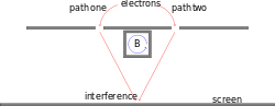
Aharonov-Bohm effect is a result of presence of gauge link instead of tensor field in the action.

Update: Gauge Invariants
Our introduction of Wilson lines (Wilson loops as well) does not depend on specific dynamics (given by an action). In reality, a dynamical theory is important for discussion of quantization, hence for quantum Wilson lines. The action of the theory has to be gauge invariant. We have already had gauge covariant quantities, the "colored" field $\phi(x)$, and the covariant derivative $D_\mu$. But we want gauge invariants/covariants involving only the gauge field to close the theory. $\left[ D_\mu, D_\nu \right] = ig F_{\mu \nu}$ is such a covariant quantity. To get gauge invariants, one simply takes $\frac{1}{2}\text{tr} F^{\mu\nu}F_{\mu\nu}$. This term is called Yang-Mills.

Wilson loop is another gauge invariants involving pure gauge field. It can also be used to construct an action. But, just as we have shown above with Stokes theorem, Wilson loops is equivalent to Yang-Mills plus other non-linear terms of it. Non-linear terms (Yang-Mills is non-linear in non-abelian gauge symmetries) are plausible in non-linear optics for example. In lattice gauge theory, Wilson loop is actually used as the action.

$\tilde{F}^{\rho\lambda} \equiv \frac{1}{2}\epsilon^{\mu\nu\rho\lambda}F_{\mu\nu}$ is also gauge covariant. But $\text{tr}\tilde{F}^{\mu\nu}\tilde{F}_{\mu\nu} = \text{tr}F^{\mu\nu}F_{\mu\nu}$. $\text{tr} \tilde{F}^{\mu\nu}F_{\mu\nu} = \frac{1}{2} \epsilon^{\mu\nu\rho\lambda}F_{\mu\nu}F_{\rho\lambda}$ is a gauge invariant. Such a term is called $\theta$-term in QCD.

In (2+1)-dimension (not limited to Minkowski space), we also have, $$\frac{k}{8\pi} \int_{\mathcal{M}} \mathrm{d}^3x \epsilon^{\alpha\beta\gamma} \text{tr}\left\{ A_\alpha (\partial_\beta A_\gamma - \partial_\gamma A_\beta)  + \frac{2}{3} A_\alpha \left[ A_\beta, A_\gamma \right] \right\}$$ This term is called Chern-Simons. $k$ is an integer for quantized theory. Chern-Simons is an important theory, because it is metric free. Such a theory is called a topological quantum field theory. Wilson loops, also metric free, are the primary observables in Chern-Simons theory.





[1]: N. E. Bralic, Phys. Rev. D 22 (1980) 3090

Some notes on non-abelian gauge theory

Non-Abelian Gauge Theory Lecture Notes, Based on Srednicki §24 & §69 

This is the lecture notes I used for this week's lecture of PHYS 682. We ended up to Yang-Mills Lagrangian, $$\mathcal{L}_\text{YM} = -\frac{1}{4} F^{\mu\nu a}F_{\mu\nu}^a + \bar\psi_i \left( i \gamma_\mu D^\mu_{ij} - m \delta_{ij} \right) \psi_j$$ where $D^\mu_{ij} = \partial^\mu \delta_{ij} - i g A^{\mu a} \tau^a_{ij}$ is the gauge covariant derivative; $F^{\mu\nu a} = \partial^\mu A^{\nu a} - \partial^\nu A^{\mu a} + g f^{a b c}A^{\mu b} A^{\nu c}$ is the field tensor.

The Secret Formula for Love

Mathematica code:

(* a xkcd-style graph converter from http://mathematica.stackexchange.com/questions/11350/xkcd-style-graphs 
by Simon Woods *)

xkcdStyle = {FontFamily -> "Comic Sans MS", 16};

xkcdLabel[{str_, {x1_, y1_}, {xo_, yo_}}] := 
  Module[{x2, y2}, x2 = x1 + xo; y2 = y1 + yo;
   {Inset[
     Style[str, xkcdStyle], {x2, y2}, {1.2 Sign[x1 - x2], 
      Sign[y1 - y2] Boole[x1 == x2]}], Thick, 
    BezierCurve[{{0.9 x1 + 0.1 x2, 0.9 y1 + 0.1 y2}, {x1, y2}, {x2, 
       y2}}]}];

xkcdRules = {EdgeForm[ef : Except[None]] :> 
    EdgeForm[Flatten@{ef, Thick, Black}], 
   Style[x_, st_] :> Style[x, xkcdStyle], 
   Pane[s_String] :> 
    Pane[Style[s, xkcdStyle]], {h_Hue, l_Line} :> {Thickness[0.02], 
     White, l, Thick, h, l}, 
   Grid[{{g_Graphics, s_String}}] :> Grid[{{g, Style[s, xkcdStyle]}}],
    Rule[PlotLabel, lab_] :> Rule[PlotLabel, Style[lab, xkcdStyle]]};

xkcdShow[p_] := 
 Show[p, AxesStyle -> Thick, LabelStyle -> xkcdStyle] /. xkcdRules

xkcdShow[Labeled[p_, rest__]] := 
 Labeled[Show[p, AxesStyle -> Thick, LabelStyle -> xkcdStyle], 
   rest] /. xkcdRules

(* Mathematica Version 8.0+ *)
xkcdDistort[p_] := 
  Module[{r, ix, iy, rand}, 
   r = ImagePad[Rasterize@p, 10, Padding -> White];
   {ix, iy} = 
    Table[RandomImage[{-1, 1}, ImageDimensions@r]~ImageConvolve~
      GaussianMatrix[10], {2}];
   ImagePad[
    ImageTransformation[
     r, # + 15 {ImageValue[ix, #], ImageValue[iy, #]} &, 
     DataRange -> Full], -5]];

(* for Mathematica version < 7 *)
xkcdDistort[p_] := 
 Module[{r, id, ix, iy, samplepoints, funcs, channels},
  r = ImagePad[Rasterize@p, 10, Padding -> White]; 
  id = Reverse@ImageDimensions[r];
  {ix, iy} = Table[ListInterpolation[ImageData[
      Image@RandomReal[{-1, 1}, id]~ImageConvolve~GaussianMatrix[10]]], {2}]; 
  samplepoints = Table[{x + 15 ix[x, y], y + 15 iy[x, y]}, {x, id[[1]]}, {y, id[[2]]}]; 
  funcs = ListInterpolation[ImageData@#] & /@ ColorSeparate[r]; 
  channels = Apply[#, samplepoints, {2}] & /@ funcs; 
  ImagePad[ColorCombine[Image /@ channels], -10]]


xkcdConvert[x_] := xkcdDistort[xkcdShow[x]]


(* the heart plot *)

xkcdConvert[
 ContourPlot[x^2 + (y - (x^2)^(1/3))^2 == 1, {x, -1, 1}, {y, -1, 2}, 
  ContourStyle -> {Red, Thick}, ContourShading -> Red, 
  AspectRatio -> 1, ImageSize -> 400, Axes -> True, Frame -> False, 
  AxesLabel -> Map[Text@Style[#, 20, Italic] &, {"x", "y"}], 
  AxesStyle -> FontSize -> 15, 
  Epilog -> {Inset[
     Style[x^2 + (y - (x^2)^(1/3))^2 == 1, Medium, Italic], 
     Offset[{0, 0}], Scaled[{-0.1, -5.5}], 1], 
    Inset[Style["xkcd-style graph", xkcdStyle, FontSize -> 12 ], 
     Scaled[{0.15, 0.05}], Automatic]}, 
  PlotLabel -> 
   Style["The Secret Formula for Love", xkcdStyle, 
    FontSize -> 24]]]

Cisco AnyConnect Client was not able to establish connection ...

I installed and used Cisco AnyConnect for a while and then suddenly one day, I cannot make a connection. The prompted error information is as following,

The Cisco troubleshooting website just told me to retry, not helpful at all. After some googling, it seems the trouble is caused by incompatibility of AnyConnect client and Windows network and file sharing service. But I have my network and file sharing option disabled already. This post suggests, not only the network and file sharing option in network and sharing center has to be disabled, but also the Internet Connection Sharing (ICS) service has to be shut down. It can be done via the following steps: find

start -> services.msc -> Internet Connection Sharing 

and disable it. (The following prompt windows is in Chinese, but similar to ones of other languages)