Faster Mathematica II: List Manipulation

The most important datatype in math is list. Lists in Mathematica are like set in mathematics. List is also used to hold data. In the case of large amount of data in input/output or intermediate stage, fast list operations certainly would speedup the code. One surprising fact is, seemly the same list operations may have different performance.

1. List Construction

1-0 Table is fast when creating block list

The most simple way to construct a list is use Table. Table[] is the suitable choice in generic cases. But making use of knowledge of the list, you can get better performance.

Table[], Array[], and function apply

1-1 use build-in functions

Some build-in functions support generation of a list. They are usually faster that explicit call them in a list constructor like Table[].  

Build-in random number generator is way faster.

1-2 use Reap-Sow, instead of Insert, Append, AppendTo, Prepend or PrependTo

1-3 Use NestList for recursable list  

Recursable list means you can get the n+1-th from the n-th. 

2. List Traversal

2-1. Listable attribute

Many function as Listable attribute. This means, when hitting a list, the function automatically hit on each element of the list. And the result will be the list of all hits. Using Listable functions is the fastest  list traversal. 

One can also Map (/@), Apply (@@, @@@), Thread, MapThread the function (head) to a list if Listable attribute is not available. 

Note that some binary operations have been defined between lists and between list and scalar. This build-in operations between lists are fast and can be in parallel. 

2-2. iterate a list

If one has to explicitly traverse a list,  Mathematica allows iterating a list directly. It is faster than using iterators. The iteration concept is not limited to list. In Do and other iterating cases, list can also be iterated directly. 

 2-3. use build-in list manipulation

Mathematica has defined many build-in list operations. Using these build-in operations are generally faster. 

Faster Mathematica I: script and text based interface

I am not a Mathematica developer, expert or advanced user. Yet I do have been using Mathematica frequently for several years. And I do know there are often slower and faster ways of using Mathematica. In these posts, I'll present my experience of Mathematica, which may or may not be the best/smart ways. I welcome the dear readers posting their experience/comments.

I have several Mathematica available, i386, x86_64 desktop and network licenced math on x86_64 supercomputer. By default, my Mathematica is running on Ubuntu/Linux i386, Mathematica for students version 8.0. Throughout these posts, I'm gonna use math for short of Mathematica.

1. Use MathKernel

The FrontEnd (in most cases, the notebook) can be very slow when there are lots stuff in it. Output data, graphs and syntax highlight may take huge amount of memory, which slows down math. In other times, the user uses math on a remote machine. The bandwidth may limit the use of FrontEnd. In either case, the user may want to interact with math kernel directly. math/MathKernel can be viewed as a text based interface of math, or an interactive version of script.

To start MathKernel, in any terminal enter math or MathKernel. To quit from math kernel, one has to use math function Exit[ ] or Quit[ ]. It also works without square bracket like Exit or Quit. Warning, enter mathematica will open a FrontEnd.

use MathKernel

2. Use math script

When working on heavy tasks, or with a queue job submission system, non-interactive scripts are often very useful. Conventionally, Mathematica packages and other Mathematica scripts end with the extension ".m", although this is not a strict requirement.

To run a math script foo.m,

math -script foo.m
or
MathKernel -script foo.m
or
math -noprompt -run "<<foo.m"

Math scripts can also be wrapped as normal executive scripts.

This is done by invoking MathematicaScript interpreter at the very beginning. The rest of the file is Mathematica commands. The interpreter line starts with two characters “#!”, following with the absolute path to the MathematicaScript interpreter. A typical script file looks like:

There is a known bug (not fixed at least in 8.0) that the MathematicaScript interpreter malfunctions in 32-bit machines.

The issue can be partially solved by using math or MathKernel as interpreter. But math or MathKernel does NOT take command line parameters (See example below).

references:
[1]: http://reference.wolfram.com/mathematica/ref/program/MathKernel.html
[2]: http://reference.wolfram.com/mathematica/tutorial/MathematicaScripts.html
[3]: http://www.wolfram.com/mathematica/new-in-8/mathematica-shell-scripts/

GNU screen: run interactive scripts in background

I have an old laptop at home. It's too slow to do any actual computing. So when I'm too lazy to go to my office, I have to ssh my desktop in my office. There is always a problem however, ssh may be time-out when I was running a long task. I could in principle, install a job schedule system, like pbs, condor. But I really wanna run interactive scripts or even X-windows on my desktop. The solution is gnu screen.

screen is a muliplexer. It's the shell version of "windows" (not confused with Microsoft Windows). It manages multiple shells (called screens) in background. The screens can be detached from your current shell, and will not stop even if the current shell terminates.

To start a new screen, one can either,

• type in screen, one enter the new screen immediately;
• <ctrl +a ctrl + c>, to create a new screen;
• screen cmd will run the command cmd in a new screen;

To detach the shell from current prompt, one can press <ctrl + a + d>.

To resume a screen, one may,

• type in screen -r [ID]; ID is needed if multiple shells are hidden. It will prompt of course all available screen IDs.

To manage multiple screens, see man screen. 

With GNU screen, I can ssh to my desktop, and use screen to run an interactive script or a program, then I detach the screen, and logout from my desktop. After sometime, I login and resume my screen to check the calculation result.;

Schroedinger's cat is a normal cat

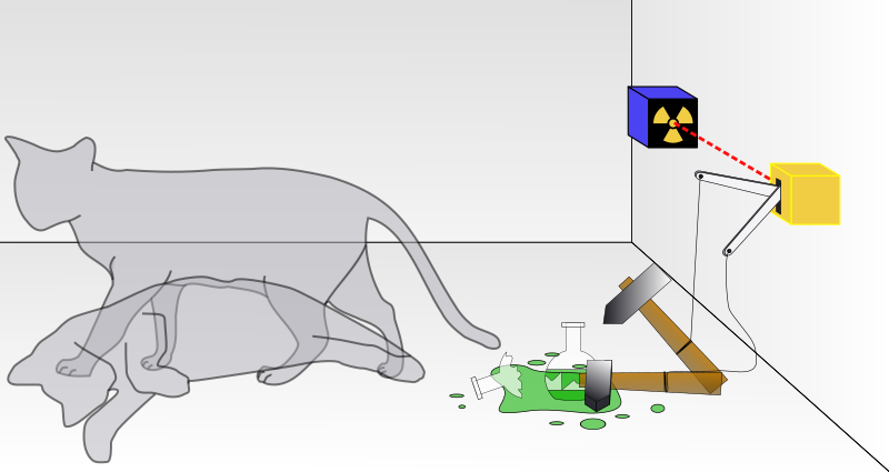
Schroedinger's Cat thought experiment is an extreme example of applying quantum mechanics to macroscopic objects, where naive quantum mechanics interpretation appears to contradict common sense.

Schrödinger's Cat: A cat, a flask of poison and a radioactive source are placed in a sealed box. If an internal monitor detects radioactivity, the flask is shattered, releasing the poison that kills the cat. The Copenhagen interpretation of quantum mechanics implies that after a while, the cat is simultaneously alive and dead. Yet, when we look in the box, we see the cat either alive or dead, not both alive and dead.

The textbook interpretation ( Copenhagen interpretation ) says, the cat+radioactive source is in an entangled state until one opens the box (measurement):
\[
\left.| \text{system} \right> = \frac{1}{\sqrt{2}} \left( \left.| : ) \right> \left.| 0 \right> + \left.| :( \right> \left.| 1 \right> \right)
\]
Entanglement implies the cat is both alive and dead before the box opened. But the application of quantum entanglement to a macro object, here cat, is controversial. In fact, the purpose of Schroedinger is to illustrate that quantum state (eps. wavefunction) may not be legitimate for describe macro system.

It's undoubted that there is something we don't know in the box, due to the quantum nature of radioactivity. But lack of information should be distinguished from quantum uncertainty.  In the sense of classical information theory, Schrodinger's cat is merely a normal cat. It's in some definite state (alive or dead). Yet different observers have different information: the experimenter said I don't know; while the flea on the back of the cat (or the cat itself) clearly knows what happened. There are many things in this world we don't know. A lot of them are associated with some quantum mechanical object (such as atoms emitting light). But we don't say, they are entangled.

It might be possible some day, the classical uncertainly and the quantum uncertainly are unified in a weird way, just like many other interpretation of quantum mechanics hoped. But in Schroedinger's Cat experiment, they are different. The main point is that the classical uncertainty is artificial. The cat is a macro object, meaning that it has huge amount of particle exchange with the environment. Outside the box, we can hear for example its scratch  sound. It's possible that the sound wave is overwhelmed by the noise, or our ears are not good enough. In either case, there exists a threshold $E_c$. Let's assume the cat-poison-radioactivity can be treated in a quantum mechanical way (See the Feynman diagram below). We can calculate the amplitudes $\mathcal{T}_{fi}$.

Notice that the cat must have interaction with the environment, we must also include such diagrams:

The sound etc. made by the cat is  characterized by $E$, $E_c$ is the threshold of the detector. 

The correction has similar structure with QED soft bremsstrahlung. In fact, we can assume the interaction of cat via environment is via QED ( for example, we can put a charge on the cat, and detect the electric field stirring outside the box). Let's simply borrow QED soft bremsstrahlung correction formula:
\[
 T'_{fi} = T^{(0)}_{fi} \cdot \exp\{ - f ( E / E_c) \}
\]
where $f(x)$ is increasing function.

The meaning of the result is, for a macro object, the correction always exist. In the case of an infinitely accurate detector, the classical cat and quantum cat cannot be distinguished by experiment. However, the amplitude is zero, i.e. still we can distinguish the classical cat and the quantum cat.