Oct 8, 2016

Numerical Solutions of the Non-Relativistic Yukawa Theory

The Yukawa potential (aka. screened Coulomb potential) $V(r) = -(\alpha/r) \exp(-\mu r)$ is a universal potential for interactions mediated by massive particles in the non-relativistic limit. It is also useful for describing interactions in the medium -- the "screened Coulomb interaction". Thus it is very important to find the solutions for the Yukawa potential in non-relativistic Schroedinger equation: \[
\Big[ -\frac{\nabla^2}{2m} - \frac{\alpha}{r} e^{-\mu r} \Big] \psi(\vec r) = E \, \psi(\vec r),
\] where $m$ is the reduced mass, $\alpha \equiv g^2/(4\pi)$ is the strength of the interaction with $g$ the "charge", $\mu$ is the mass of the exchanged particle, and $\mu=0$ gives the Coulomb potential. Alas, the above eigenvalue problem does not admit analytic solution, except for the Coulomb case. This post describes a numerical method for solving Schroedinger equation with the Yukawa potential.

Fig. 1: Feynman diagram of a boson (wavy line) mediated interaction.

In the momentum space, the eigenvalue equation becomes an integral equation: \[
\frac{\vec p^2}{2m} \psi(\vec p) - \int \frac{\mathrm{d}^3 p'}{(2\pi)^3} \frac{4\pi \alpha}{(\vec p-\vec p')^2+\mu^2} \psi(\vec p') = E\,\psi(\vec p).
\] Here $\psi(\vec p)$ represents the momentum-space wave functions, related to the coordinate-space wave function $\psi(\vec r)$ by a Fourier transformation, \[
\psi(\vec p) = \int \mathrm d^3r \, e^{i \vec p\cdot \vec r} \psi(\vec r). \\
\psi(\vec r) = \int \frac{\mathrm d^3 p}{(2\pi)^3} \, e^{-i \vec p\cdot r} \psi(\vec p).
\] We have abused the notation $\psi$ for wave functions. The wave functions should be normalized according to \[
\int \mathrm d^3 r\, \psi^*(\vec r) \psi(\vec r) = 1, \\
\int \frac{\mathrm d^3 p}{(2\pi)^3} \psi^*(\vec p) \psi(\vec p) = 1.
\]

Dimension Reduction

Before employing numerical methods, let us first put the equation to a dimensionless form. The natural scale in the problem is the Bohr radius ($\hbar = c = 1$): $a \equiv 1/(\alpha m)$. We also define: $\lambda \equiv a\mu$, $\kappa \equiv 2 m E a^2 = 2 E/ (m \alpha^2) \equiv E / E_B$, with $E_B \equiv \frac{1}{2} \alpha^2 m$ being the ground state energy (binding energy) of the Coulomb theory (such as the Hydrogen atom, positronium and so on), and $\vec p \to a \vec p$, $\vec r \to \vec r/a$. Then, the equations becomes, \[
\Big[ - \nabla^2 - \frac{2}{r} e^{-\lambda r} \Big] \psi(\vec r) = \kappa \, \psi(\vec r), \\
\vec p^2 \psi(\vec p) - \int \frac{\mathrm d^3 p'}{(2\pi)^3} \frac{8\pi}{(\vec p - \vec p')^2 + \lambda^2} \psi(\vec p') = \kappa \, \psi(\vec p).
\] The theory has a rotational symmetry and the wave functions can be written as, \[
\psi(\vec r) = R(r) Y_{lm}(\hat r), \quad \psi(\vec p) = \phi(p) Y_{lm}(\hat p).
\] $Y_{lm}$ are the spherical harmonics. They are the eigen function of the angular momentum squared operator $\vec L^2$. Therefore, we only need to solve for the radial part $R(r)$ or $\phi(p)$. They are related by a Hankel transformation: \[
R(r) = \frac{(-i)^\ell}{8\pi^3} \int_0^\infty \mathrm dp \, p^2 j_\ell(pr) \phi(p), \\
\phi(p) = i^\ell \int_0^\infty \mathrm dr \, r^2 j_\ell(pr) R(r).
\] $j_\ell(z)$ is the spherical Bessel function of the first kind. $Y_{lm}$ are normalized: \[
\int \mathrm d^2\Omega(\hat r) Y^*_{l'm'}(\hat r) Y_{lm}(\hat r) = \delta_{ll'}\delta_{mm'}.
\] Similarly, the radial wave function are normalized according to: \[
\int_0^\infty \mathrm d r \, r^2 R^2(r) = 1, \\
\frac{1}{8\pi^3} \int_0^\infty \mathrm d p\, p^2 \phi^2(p) = 1.
\]

Coordinate Space

The coordinate-space Schroedinger equation can be written in the spherical coordinates: \[
\Big[ - \frac{1}{r^2}\frac{\partial }{\partial r}\big( r^2 \frac{\partial }{\partial r} ) + \frac{l(l+1)}{r^2} - \frac{2}{r} e^{-\lambda r} \Big] R(r) = \kappa \, R(r). \\
\Leftrightarrow \Big[- \frac{\partial^2 }{\partial r^2} + \frac{l(l+1)}{r^2} - \frac{2}{r} e^{-\lambda r} \Big] u(r) = \kappa \, u(r),
\] where $u(r) = r R(r)$.

The above differential equations can be discretized and solved numerically. In this post, however, we will focus on the momentum space representation and its numerical solutions.

Momentum Space

In the momentum space, Schroedinger equation can be written as \[
p^2 \phi(p) - \frac{4}{\pi} \int_0^\infty \mathrm dp' \, p'^2 K_\ell (p, p') \phi(p') = \kappa \, \phi(p),
\] where \[
K_\ell(p, p') \equiv \int_0^\infty \mathrm dr \, r \exp(-\lambda r) j_\ell(pr) j_\ell(p' r).
\]
Here are the analytical expressions for the first few $K_\ell$: \[
\begin{split}
(S\text{-wave})\quad K_0(p, p') =& \frac{1}{4 pp'}\log \Big[\frac{(p+p')^2+\lambda^2}{(p-p')^2+\lambda^2}\Big]; \\
(P\text{-wave})\quad K_1(p, p') =& \frac{p^2+p'^2+\lambda^2}{4 p^2p'^2}\log\Big[\frac{(p+p')^2+\lambda^2}{(p-p')^2+\lambda^2}\Big]-\frac{1}{2pp'}\\
(D\text{-wave})\quad K_2(p, p') =& \frac{3p^4+2p^2p'^2+3p'^4+6(p^2+p'^2)\lambda^2+3\lambda^4}{16p^3p'^3}\log\Big[\frac{(p+p')^2+\lambda^2}{(p-p')^2+\lambda^2}\Big]
- \frac{3(p^2+p'^2+\lambda^2)}{8p^2p'^2}\\
\vdots&
\end{split}
\] In the general case, $K_\ell$ can be evaluated numerically using quadrature method.

We can use the quadrature method to approximate the integral. For a general integral, \[
\int \mathrm dx \, f(x) = \sum_{i=1}^N w_i f(x_i) + R[f^{(2N+1)}(\xi)]
\] where $x_i$ and $w_i$ are pre-chosen abscissas and weights. For the radial integral, we can use the Gauss-Legendre quadrature with a mapping function: \[
\theta: (-1, +1) \to (0, \infty); \\
r_i = \theta(x^\text{gl}_i), \quad w_i = w^\text{gl}_i \theta'(x_i)
\] where $x^\text{gl}_i$, and $w^\text{gl}_i$ are the standard Gauss-Legendre quadrature abscissas and weights.

While in principle the converged result is independent of the mapping function, the choice of the mapping function is very important in practice, as it controls the rate of convergence. It should be chosen to cover the extent of the wave function. Because different states have different radial extent, it is often difficult to come up with a universal mapping function optimal for all excited states. Fortunately, in most practical cases, we are interested in the first lowest states.  Common choices include (first, $x$ is mapped to $(0,1)$ ): $r = x/(1-x)$, $r=a \tan (x \pi/2)$, $r = a (1-e^{-bx})/(e-e^x)$ ...

The integral equation becomes, \[
p^2_i \phi(p_i) - \frac{4}{\pi} \sum_j w_j p^2_j K_\ell (p_i, p_j) \phi(p_j) = \kappa \, \phi(p_i).
\] It is convenient to define $v_i \equiv \sqrt{w_i} p_i \phi(p_i)$, with normalization \[
\sum_i v_i^2 = 1.
\] Then, the discretized equation becomes, \[
\sum_j H_{ij} v_j = \kappa \, v_i,
\] where the Hamiltonian matrix $H_{ij}$ reads, \[
H_{ij} = \delta_{ij} p^2_i - (4/\pi) \sqrt{w_i w_j} \, p_i p_j \, K_\ell (p_i, p_j).
\] $H$ is obviously Hermitian. The energy eigenvalue and the wave functions can be obtained by numerically diagonalizing the Hamiltonian matrix.


Fig 2: Visualization of the Hamiltonian matrix, $\ell = 0$ (S-wave), quadrature order $N=512$.


The system can be solved in different quadrature order. The continuum limit can be reach by extrapolating the quadrature order $N\to\infty$.

Energy Eigenvalues 

The obtained energy eigenvalues as a function of the exchanged particle mass $\mu$ are shown in Fig. 3. At small $\mu$, the binding energies approach to the standard Coulomb values $E_n^{(\text{coul})}=-\alpha^2 m / (2n^2)$ where $n=1,2,3,4,\cdots$ is the principle quantum number. The ground state energy is also in good agreement with the upper bound obtained from the variational method, using the Coulomb wave function as trial functions. As $\mu$ increases, bound states gradually disappear. Even the ground state dissociates as $\mu \gtrsim \alpha m$.


Fig. 3: The S-wave energy eigenvalues as a function of $\mu$. The values are obtained by extrapolating results over quadrature grids of the order $N=16, 32, 64, 128, 512, 1024$. The red crosses represent Coulomb energy levels $E_n^{(\text{coul})} = - \alpha^2 m/(2n^2)$, $n=1,2,3,\cdots$. The red dashed line represents the upper bound obtained from variational method, using the Coulomb wave function as trial functions.

Wave Functions

Fig. 4: The obtained ground state S-wave momentum-space wave functions for selected $\mu$.

The momentum-space wave functions can be extracted from the obtained eigenvectors (see Fig. 4 and 5). At small $\mu$, the wave functions approach to the Coulomb result. As $\mu$ increases, the wave function within the momentum space becomes narrower. Furthermore, the change in excited wave functions are more dramatic comparing to the ground state wave function as $\mu$ increases.


Fig. 5: The obtained radially excited S-wave momentum-space wave functions for selected $\mu$.


.

Jul 3, 2015

Gravity in the 2+1 dimensions

In a previous post, we point out in the d+1 dimensions, the Coulomb's law reads, \[
\varphi(r) = \frac{\Gamma(\frac{d-2}{2})}{4\pi^{\frac{d}{2}}}\frac{1}{r^{d-2}}.
\] Apparently, in the 2+1 dimensions, this formula is divergent. To see this, first note that $x^\epsilon = 1 + \epsilon \log x$, and $\Gamma(\epsilon) = 1/\epsilon - \gamma$, the potential reads, \[
\varphi(r) \triangleq \lim_{\epsilon\to 0^+} \frac{\Gamma(\frac{\epsilon}{2})}{4\pi^{\frac{2+\epsilon}{2}}}\frac{1}{r^{\epsilon}} = \frac{1}{2\pi}\log\frac{1}{r} + \frac{1}{2\pi\epsilon} - \frac{1}{4\pi}\log e^\gamma\pi
\] We can regularize the potential by adding an infinitely large constant such that it obtains a finite value at a given distance $r_0$: \[
\varphi_r(r) = \frac{1}{2\pi}\log\frac{r_0}{r}.
\] But still, the potential divergences at infinity, which sort of violates the spirit of "locality".

The interpretation of this mathematical phenomenon is that in the 2+1 dimensions, long range correlation can be created with infinitely small energy. A consequence of this is the Coleman's theorem, stating that there is no spontaneous symmetry breaking of the continuous symmetry in the 2 dimensions.

In terms of the gravity, this infrared divergence is obviously non-physical. The potential becomes infinitely large near the source and far away from the source. A plausible interpretation is therefore $\varphi = \text{constant}$, at least for the type of gravity as we understand (We are not claiming the Poisson equation has no non-trivial solution in 2 dimensions.).

Of course, with a strong field strength, Newton's law should be replace by Einstein's equation: \[
R_{\mu\nu}  =  8\pi G \Big( T_{\mu\nu} - T g_{\mu\nu} \Big).
\] Here $T = g^{\mu\nu} T_{\mu\nu}$. In the vacuum, this equation reduces to $R_{\mu\nu} = 0$.  But this does not necessarily mean the space-time curvature is zero. The space time curvature is ultimately determined by the Riemann tensor $R^\mu_{\nu\sigma\rho}$. Non-vanishing curvature represents the propagation of the gravity from the source inside the vacuum.

Riemann tensor has $D^2(D^2-1)/12$ independent components, where $D=d+1$ is the space-time dimensionality. In the 2+1 case, it has 6 independent components, whereas the Ricci tensor $R_{\mu\nu}$ has $(3 \times 3 +3)/2 = 6$ independent components as well. Thus, Riemann tensor is expressible through the Ricci tensor: \[
R_{\mu\nu\rho\sigma} = \big( g_{\mu\rho}R_{\nu\sigma} - (\rho \leftrightarrow \sigma) \big) - (\nu \leftrightarrow \rho) - \frac{1}{2} (g_{\mu\rho}g_{\nu\sigma} - g_{\mu\sigma}g_{\nu\rho}) R
\] Here $R = g^{\mu\nu}R_{\mu\nu}$. As a result, Riemann tensor, hence the space-time curvature, is zero in the vacuum, in the 2+1 dimensions. This means gravity cannot propagator through the free space in the 2+1 dimensions! Einstein's equation is a full pledged dynamical theory of gravity with Newton's gravitational theory as its weak field approximation. Now, Einstein's theory actually agrees with Newton's theory that in the 2+1 dimensions there is no gravity!

Applying the gravitational theory in the 3+1 dimensions into the 2+1 dimension is somewhat unjustified. After all, non-body knows wether these are the correct modeling. However Newton's law is not an ad loc construction. It follows, as the Coulomb's law, the Poisson equation $\nabla^2 \varphi(x) = 0$. Einstein's equation has a stronger built-in beauty in it: it acquires a geometric interpretation. So these interesting observation is not a major consequence of our gravitational theory per se. It is more closely related to the special topology of the low dimensions, which is also well known. In fact, in the 2 dimensions, topology is more central than the local operators we cherish much in the 3 dimensions.


Apr 14, 2015

Everything Seems Linear in the Log Scale

Figure: the Standard Model fermion mass hierarchy shown in the log scale.

Apr 4, 2015

The Super Critical Charge


Schwinger Effect

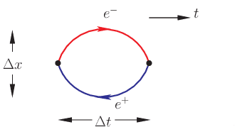
According to quantum field theory, vacuum, the state of no nothingness, is actually filled with virtual particles. In particular, virtual electron and positron pairs are created and annihilated in short time and distance: \[
\Delta t \sim \frac{h}{2m_ec^2} \simeq 10^{-21} \,\mathrm{s}, \quad \Delta x \sim \frac{h}{2m_ec} \simeq 10^{-12} \,\mathrm{m}. \]
Fig. 1: Vacuum fluctuation into electron-positron pair.

Then, it is no surprise that if we exert a strong electric field $\vec E$ on the vacuum, the virtual electron and positron would be pulled in the opposite direction. As a net result, real electron and positron pairs can be created out of vacuum. Of course, the electric field has to be strong, to provide enough energy ($\gtrsim 2m_e c^2$) for the pair production. We can do an estimation as following. In order to create real particles, the electron and positron have to be pulled apart by at least one Compton length $\lambda_e = \frac{\hbar}{m_e c}$ (so that their wave packets do not overlap much). Over such a distance, the energy provided by the electric field is, $e E \lambda_e \ge 2 m_e c^2$. Therefore the threshold electric field is \[
E_\mathrm{th} \triangleq \frac{2 m_e c^3}{e\hbar} \simeq 10^{18} \, \mathrm{V/m}.
\]

Fig. 2: The Schwinger effect.
We can also look at the problem in another way (Fig. 2). In the Dirac theory, the vacuum is filled with negative energy electrons, known as the Dirac sea. In order to become physical, the electron has to get to the positive mass shell $E = \sqrt{\vec p^2 c^2 + m^2c^4}$. There is a $2 m_e c^2$ mass gap between them. (The Coulomb potential is negligible comparing to the mass gap.)

Fig. 3: The mass gap. The $x$-axis is the separation between the electron and its hole. Due to zitterbewegung, this distance can not be smaller than the Compton length.

Therefore, the creation of an electron (and the positron - the hole in the Dirac sea) can be viewed as a quantum tunneling process (Fig. 3). Then the external electric field turns the well to a barrier. The width of the barrier is proportional to $w \sim 2 m_e c^2/E$. According to WKB, the tunneling probability is \[
P \sim \exp\Big( - w \sqrt{2 m_e \times e (2m_e c^2) } \Big) \simeq \exp\Big( - E_\mathrm{th}/E \Big)
\]

Fig. 4: The electric field term the mass well to a barrier.

Super Critical Charge

We have seen in the last section that strong electric field can create electron-positron pairs out of vacuum. The Coulomb potential have a field strength proportional to $1/r^2$: $eE(r) = \frac{Z\alpha}{\hbar c r^2}$. Very close to the charge, the electric field would be extremely intense. So, it is natural to ask, if/why not such a phenomenon can be seen around a point charge. To achieve the threshold strength, the distance $r_\mathrm{th} = \sqrt{\frac{1}{2}Z\alpha} \lambda_e \simeq \sqrt{Z/2} \times 10^{-13}\,\mathrm{m}$ has to be large than the smallest distance between two particles.

For poin-like charged particles, such as electron, muons, the smallest distance is determined by 1). their Compton wavelength (zitterbewegung) $\lambda_\ell = \frac{m_e}{m_\ell}\lambda_e$; 2). the size of the bound state $\frac{m_\ell}{m\ell+m_e}\lambda_e/(Z\alpha)$. For electron/positron, this distance $r_\mathrm{th} = \sqrt{\alpha/2} \lambda_e$ is much smaller than their Compton wavelength. Therefore, even if such a phenomenon exists, it is included in the quantum fluctuation of the particle itself. Muon is about 207 times heavier than the electron. So its Compton wavelength is 207 times smaller than electron's. Then it is possible to produce a pair of real electron-positron. But as the pair were produced, the positron would be bound with the muon, forming a $\mu^-e^+$ atom.  However, the ground state radius of this atom $r \simeq a_0 = \lambda_e / \alpha \gg r_\mathrm{th}$. In other words, there is no enough energy to produce the electron-positron pair.  Similar cases happen for other leptons.

Fig. 5: The electron-positron pair production by a muon. This process is kinematically forbidden.

For composite systems, the charge factor $Z$ can be rather large. As a result, the possible bound state radius would decrease and the threshold radius increase (while the Compton wavelength remains the same). At some critical charge factor $Z_c \simeq 2/\alpha = 274$, the system would have enough energy to produce the electron-positron pair.

Again, Dirac Sea

To give a little bit quantitative touch, let's turn to the Dirac theory again (We don't turn to Schroedinger's theory because at the super critical charge, the system is relativistic.). The Dirac equation with a Coulomb potential produces the energy spectrum (Sommerfeld fine-structure formula): \[
E_{n,j} = mc^2 \left[ 1 + \frac{Z^2\alpha^2}{\left[n-j-\frac{1}{2} + \sqrt{(j+\frac{1}{2})^2-Z^2\alpha^2}\right]^2} \right]^{-1/2}
\] where $n = 1, 2, 3, \cdots$ is called the principal quantum number and $j=1/2, 3/2, 5/2, \cdots n-1/2$ is the total angular momentum. As we can see, for the S-state ($j=1/2$), the energy becomes imaginary if $Z > 1/\alpha \simeq 137$. This is half of the critical charge we found above using a crude estimate.

The existence of imaginary energy eigenvalues implies the Dirac Hamiltonian is no longer Hermitian as Dirac promised. Something is wrong. The solution of the Dirac equation does not represent the motion of an electron. Instead, given the time-dependent part $\exp\big(- |E|t \big)$, it represents the amplitude of some tunneling process.

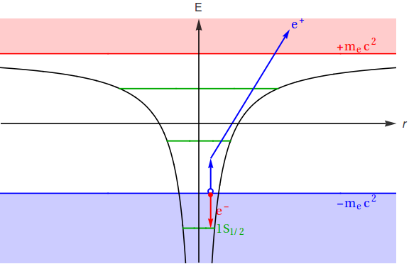
Even though Dirac's theory is broken at $Z>137$, we can still mill some plausible physics out of it, invoking the Dirac sea -- as one may have noted, the creation of particles in the Dirac theory always involves the Dirac sea. It turns out, at the presence of the super critical charge, the Coulomb level dives into the Dirac sea. Therefore, the electrons at the Dirac sea jump down to Coulomb levels below and leave holes in the Dirac sea, manifested as the positron (see Fig. 6). This interpretation can be elaborated (including using other methods) to give the semi-quantitative dynamics of the process.

Fig. 6: The Dirac interpretation of the electron-positron pair production by a super critical charge.

QED with Strong External Fields

This problem can also be described by QED. Unlike the Dirac theory, the QED Hamiltonian is always Hermitian. Hence a self-consistent quantitative description of the problem has come from QED.

In QED, the vacuum is the ground state of the charge-zero sector:\[
H_\mathrm{QED} |\Omega\rangle = E_\Omega |\Omega\rangle
\] Here $H_\mathrm{QED}$ is the QED Hamiltonian. $E_\Omega$ is the vacuum energy. It can be renormalized to 0.

In our problem, there exists a charged heavy ion $Z^+$, which generates an strong electromagnetic field $\mathcal A$. With the presence of this field, the ground state may be different: \[
\big( H_\mathrm{QED} + J_\mu \mathcal A^\mu \big) |\Omega_{\mathcal A}\rangle = E_\mathcal{A} |\Omega_{\mathcal A}\rangle
\] Where $|\Omega_{\mathcal A}\rangle$ represents the polarized QED vacuum within field $\mathcal A^\mu$, $J^\mu = e\bar\psi \gamma^\mu \psi$ is the fermion charge current.

If the charge of the heavy ion is subcritical, the polarized vacuum only involves the photon loop-correction and electron loop-corrections (see Fig. 7), which can be taken into account by renormalization (UV renormalization and the bremsstrahlung) of the heavy ion. When the mass of the heavy ion is sufficiently large, the renormalization effects can be neglected. When the charge of the heavy ion $Z^+$ exceeds some critical value $Z_c$, a new vacuum state emerges. It consists a free positron and a $Z^+e^-$ bound-state. Such a vacuum state is called a charged vacuum. Dynamically, we see the spontaneous production of an electron-positron pair.


Fig. 7: The QED vacuum within the subcritical (top) and supercritical (bottom) external field. The double line represent the heavy ion with a positive subcritical charge. The single line loop represents the electron/positron loop correction. The wavy lines represents the photons. The dot represents the coupling between the photon and the super critical charge. The blue single line represents the emitted positron. The red single line represents the bound electron.


In practice, the matrix can be truncated to the first few sector to retain the minimal physical of the charged vacuum (See Fig. 9). The minimal sector should include at least one photon and one pair of electron and positron.

Fig. 9: The QED matrix within the first few Fock sectors. The vertex with a dot represents the super critical charge coupling $Ze$.
We can further suppress the heavy ion sector and treat the field it generates simply as a classical external field. In this way the charged vacuum is more qualified for its name. (Otherwise it is just the ground state of the supercritical charge sector.)

Fig. 10: (left panel) the vacuum polarization within a subcritical potential; (right panel) the pair production (the charged vacuum) within a supercritical potential.
The charged vacuum can also be studied within the path integral formalism. According to this formalism, the vacuum expectation value of an operator within the external field is, simply, \[
\langle \mathrm T\mathcal O_\psi \rangle_{\mathcal A} = \int \mathcal D_{\psi,\bar\psi, \mathcal A} \, \mathcal O_\psi \, \exp\Big[ i\int d^4x \, \bar \psi(x) \big( i\gamma^\mu D_\mu - m\big) \psi(x)\Big]
\] where $D_\mu = \partial_\mu - ie\mathcal A_\mu$.

Both the matrix diagonalization and the path integral methods are non-perturbative. But different approximation may arise for each formalism. We shall not delve into those lengthy technologies but only mention one famous result due to Schwinger. Let's consider the production rate, which is related to the vacuum decay probability: $P = 1 - |\langle\Omega_{\mathcal A}|\Omega_{\mathcal A}\rangle|^2 \approx 1 - \exp( -2 \mathrm{Im} S_\mathrm{eff})$. Here Schwinger applied an approximation: $\langle\Omega_{\mathcal A}|\Omega_{\mathcal A}\rangle = \det^{-1} \bar\psi \big( i\gamma^\mu D_\mu - m\big) \psi \approx \exp(i S_\mathrm{eff})$. $S_\mathrm{eff}=\int d^4x\,\mathcal L_\mathrm{eff}$ is called the effective action. The one-loop effective action was calculated obtained Heisenberg and Bonn. Plug into this effective action, and assuming a uniform electric field $E$, Schwinger's conclusion for the vacuum pair production rate is, \[
R \triangleq \frac{dN}{dVdt} = \frac{(eE)^2}{4\pi^3}\sum_{n=1}^\infty \frac{1}{n^2} \exp\big( -n\pi E_c/E\big)
\] where $E_c \triangleq m_e^2 c^3/(e\hbar) \sim 10^{18} \,\mathrm{V/m}$ is the critical electric field. This formulation is the famous Schwinger mechanism of vacuum pair production.


One can also solve the Schroedinger's equation directly, starting for example, from the normal QED vacuum state: \[
 i \frac{\partial}{\partial t} |\psi(t)\rangle = \big( H_\mathrm{QED} + J^\mu \mathcal A_\mu\big) | \psi(t)\rangle, \quad
 |\psi(0)\rangle = |\Omega\rangle.
\] In this way, the time evolution of the QED vacuum can be studied. This approach is also non-perturbative.

In the above description, we deliberately avoid the photon mediated electron-positron interaction. This can be included by the quantized electromagnetic field $A^\mu$. So the full covariant derivative can be written as $D_\mu = \partial_\mu - i e\mathcal A_\mu - ie A_\mu$. Note that this field is small comparing with the external field $\mathcal A$ generated by the supercritical heavy ion, $|\mathcal A| \sim Z |A|$. In practice, the correction due to quantized photon can be included through the usual perturbation theory.

Fig. 11: the same diagrams as Fig. 10, but taking into account the quantized photons. The external fields are represented as double wavy lines. The real photon lines are the single wavy lines.

Pair Production in the Relativistic Heavy Ion Collisions


Experiments


[ To Be Continued ... ]


References:

[1]: W. Greiner, B. Muller and J. Rafelski, Quantum electrodynamics of strong fields, (1985) Springer-Verlag, Berlin Heidelberg.

Feb 23, 2015

The Year of Sheep, or Goat?

In Feb. 18, 2015, East Asians celebrated the Lunar New Year, the year of yang (羊)。 Some English media suddenly found it hard to convey the message to the English audience, as the word yang (羊) in Chinese may refer to several types of animals in English, most commonly, sheep (called mian-yang, 绵羊, in Chinese) and goat (called shan-yang, 山羊 in Chinese). So what year is it, sheep or goat?

So problem is that English does not have a collective word for sheep and goat. Scientifically speaking, the name sheep or goat itself is also a notation that refers to several similar animals. This is, of course,  very common in linguistics and may happen between any two languages. But it is not exactly true. Because there actually exists a word for animals similar to sheeps and goats: Caprinae. This is a subfamily name, which includes both sheep or ovis and goat capra. So, next time, when asked, you can tell people, IT IS THE YEAR OF CAPRINAE, if you want to be scientifically accurate.

Dec 24, 2014

The Golden-Thompson Inequality and the Upper bound of Quantum Partition Function


Let $A$ and $B$ be two Hermitian matrices. The famous Baker-Campell-Hausdorff formula says, \[
\exp\big( A + B \big) = \exp \big( A \big) \exp\big( B \big) \exp\big( - [A, B]/2 \big) \exp\big( [A, [A, B]]/6 + [B, [A,B]]/3 \big)\cdots
\] In general, $ \exp(A+B) \ne \exp (A) \exp(B) $. Applying the trace-determinant relation $\det \exp A = \exp \mathrm{tr} A$, however, we still have \[
\det\exp(A+B) = \det \exp(A) \exp(B).
\]

In a similar fashion, the Golden-Thompson theorem states, \[
\mathrm{tr}\exp(A+B) \le \mathrm{tr} \exp(A) \exp(B),
\] the equality holds iff $[A, B] = 0$.

As an application, let's consider $-\beta^{-1}A = \hat p^2/(2m), -\beta^{-1}B = V(\hat q)$, and $[\hat q, \hat p] = i$. $-\beta^{-1}(A + B) = \hat p^2/(2m) + V(\hat q) = \hat H$ is the single-particle Hamiltonian. Apparently, $Z(\beta) = \mathrm{tr} \exp( -\beta \hat H )$ is the partition function of the one-body system. Now consider the right-hand side: \[
\begin{split}
& \mathrm{tr} \exp(-\beta \hat p^2/(2m)) \exp(-\beta V(\hat q) ) \\
& = \int dq \int \frac{dp}{2\pi} \langle q | \exp(-\beta \hat p^2/(2m)) | p \rangle \langle p | \exp(-\beta V(\hat q) ) | q \rangle \\
& = \int dx \int \frac{dp}{2\pi} \exp(-\beta p^2/(2m))  \exp(-\beta V(q) )  \langle q | p \rangle \langle p | q \rangle \\
& = \int dx \int \frac{dp}{2\pi} \exp(-\beta ( p^2/(2m) + V(q)) ) \\
& =  \int dx \int \frac{dp}{2\pi} \exp( -\beta H ) = Z_\text{cl}(\beta).
\end{split}
\] The last line is the partition function of a classical single-particle system.

Therefore, the Golden-Thompson theorem says, the classical partition function is the upper bounds of the quantum partition function, $Z(\beta) \le Z_\text{cl}(\beta)$. Replace the single-particle operator and single-particle basis with the many-body ones, or even second quantized fields, it is straight-forward to show the general relation between quantum and classical partition functions.


Oct 29, 2014

Disturbing a Quantum Field

Lesson from Condensed Matter Physics (CMP)

In condensed matter systems, it is useful to study the collective response to external fields. For example, when adding an electric field $\vec E$ to a metal, a current $\vec J$ would be generated. We call the response the conductivity, which is unique for each material, thus reflects internal properties of the system. Quantitatively, the conductivity is defined in terms of the external field and the respond current \[
J(t, \vec x) = \int \mathrm d^3x' \int_{-\infty}^t \mathrm dt' \sigma(t-t', \vec x - \vec x') E(t', \vec x').
\] The upper limit of the temporal integral is due to causality. In general, the conductivity may depends on the external field $\vec E$ (non-linear effect). In the weak field limit $E \to 0$,  however, it is independent to $E$ (linear response) and provides an important probe for the property of the material. There are also other linear responses of the condensed matter systems. The Green-Kubo formula (Melville Green 1954, Ryogo Kubo 1957) provides a neat recipe to compute the linear response of the condensed matter system to an external field.

Suppose a weak external field $F(t, \vec x)$ couples to a condensed matter system through $H_\mathrm{int} = \int \mathrm d^3x F(t, \vec x) A(t, \vec x)$. The system was originally described by the density operator $\varrho =Z^{-1} \exp \big[ -\beta (H - \mu N) \big]$, where $Z = \mathrm{tr} \exp \big[ -\beta (H - \mu N) \big]$. The linear response theory concerns the expectation value of an observable $B(t, \vec x)$: \[
\langle  B(t, \vec x) \rangle_F - \langle  B(t, \vec x) \rangle= \mathrm{tr} \left[ \big(\varrho_F(t)-\varrho(t)\big) B(t, \vec x) \right] \equiv \int \mathrm dt' \int \mathrm d^3x' \chi_{AB}(t-t',\vec x-\vec x') F(t', \vec x')
\] where $\varrho_F(t)$ is the density matrix in the perturbed system. The Green-Kubo formula asserts that the linear transportation coefficient \[
\chi_{AB}(t-t', \vec x - \vec x') = -i \Theta(t-t') \langle [B(t, \vec x), A(t', \vec x')] \rangle.
\] For example, the conductivity is related to the current-current correlation function*, \[
\sigma_{AB}(t-t', \vec x - \vec x') = -i \Theta(t-t') \langle [\partial_t^{-1}J(t, \vec x), \partial_{t'}^{-1}J(t', \vec x')] \rangle.
\]

*In general, the current is a four-vector hence the response is a tensor. One should consider the contribution from all components, which gives rise to several transport coefficients: the longitudinal conductivity, the density responses as well as the Hall conductivity etc.

Quantum Field Theory (QFT)

The vacuum state of QFT $|\Omega\rangle$ is intrinsically many-body (even the free field theory!). Let's disturb the QFT vacuum and measure the linear response.


Let $J_r(x)$ be a classical source. We couple it to the quantum field $\varphi(x)$ through $\mathscr H_\mathrm{int}(x) = A_r(x) J_r(x)$, where $A$ is a local operator constructed from $\varphi$. Then we measure the vacuum expectation value (VEV) of an observable $B_s(x)$ (To measure this observable, we may, for example, couple the field to a classical field. That's why we often consider the case $A = B$, which we sill talk about later.): $\langle B_s(x) \rangle_J \equiv Z_J^{-1} \langle \Omega | B_s(x) | \Omega \rangle_J$, where $Z_J = \langle \Omega | \Omega\rangle_J$ is the perturbed partition function. In the weak source limit ($J\to 0$), the response should be linear, similar to the condensed matter system: \[
\langle B_s(x) \rangle = \int \mathrm d^4 x' \chi_{sr}^{BA}(x,x') J_r(x') + \mathcal O(J^2).
\] Let $Z$ be the unperturbed partition function. In the weak external field limit $J \to 0$, \[
Z_J = Z \Big(1 - i \int \mathrm d^4x \langle A_r(x) \Omega \rangle J_r(x) - \frac{1}{2} \int \mathrm d^4x\mathrm d^4y \langle \mathcal T\big\{ A_r(x) A_s(y) \big\} \rangle J_r(x) J_s(y) \Big).
\] and $\langle \Omega | B_s(x) | \Omega \rangle_J$ is, \[
 \langle \Omega | B_s(x) | \Omega \rangle_J = \langle \Omega | B_s(x) | \Omega \rangle
  -i \int \mathrm d^4 x' \langle \Omega | \mathcal T \big\{B_s(x)A_r(x')\big\} | \Omega\rangle J_r(x').
\] Then the vacuum expectation value (VEV) \[
\langle B_s(x) \rangle_J
= \langle B_s(x) \rangle + i \int \mathrm d^4x' \langle A_r(x') \rangle \langle B_s(x) \rangle J_r(x') - i \int \mathrm d^4 x' \langle \mathcal T \big\{B_s(x) A_r(x')\big\} \rangle J_r(x').
\] It is convenient to work with "renormalized" operators that have vanishing VEV without the presence of the external source. For example, we may define: $B^R_s(x) = B_s(x) - \langle B_s(x)\rangle$. It is easy to see,\[
\langle B^R_s(x) \rangle_J
=- i \int \mathrm d^4 x' \langle \mathcal T \big\{B^R_s(x) A^R_r(x')\big\} \rangle J_r(x').
\] Therefore, the transport coefficient $\chi(x,x') \propto \langle \mathcal T \big\{B^R_s(x) A^R_r(x')\big\} \rangle$. Note that causality is preserved by time-ordering operator $\mathcal T$.

From now on, we'll assume all the operators have been properly renormalized, unless elsewhere stated.

Example 1: Field Propagation

$A = B = \varphi$, where $\varphi(x)$ is the renormalized field such that $\langle \Omega |\varphi(x)|\Omega\rangle = 0$. $\langle\varphi(x)\rangle_J$ represents the amplitude for finding a physical particle in the disturbed vacuum. \[
\langle\varphi_a(x)\rangle_J =- i \int \mathrm d^4 x' \langle \mathcal T \big\{\varphi_a(x) \varphi_b(x')\big\} \rangle J_b(x'),
\] Here $D_{ab}(x-x') \equiv i\langle \mathcal T \big\{\varphi_a(x) \varphi_b(x')\big\} \rangle$ is nothing but the Feynman propagator. This means sense physically: the classical source $J$ creates a physical particle at $x'$, and then the particle propagate to $x$ to be detected.

Note that we are not doing perturbation theory. The graphical representations are not necessarily Feynman diagrams.

Example 2: Vacuum Polarization

Let $A = B = J^\mu(x)$, where $J^\mu$ is the electromagnetic current. We couple a classical electromagnetic field $\mathcal A_\mu(x) e^{-\epsilon |x^0|}, (\epsilon\to 0^+)$ to the vacuum and measure the current: \[
\langle J^\mu(x) \rangle_{\mathcal A} = -i \int \mathrm d^4x' \left< \mathcal T \big\{J^\mu(x)J^\nu(x') \big\}  \right> \mathcal A_\nu(x') e^{-\epsilon |x'^0|}.
\] The linear transport coefficient is called the polarization tensor: \[
\Pi^{\mu\nu}(x-x') \equiv \left< \mathcal T \big\{J^\mu(x)J^\nu(x') \big\}  \right>.
\] Consider a free Dirac field, \[
\psi(x) = \sum_{s=\pm} \int\frac{\mathrm d^3 k}{(2\pi)^32\omega_p} \Big[ u_s(k) b_s(k) e^{ik\cdot x} + v_s(k) d^\dagger_s(k) e^{-ik\cdot x} \Big].
\] The electromagnetic current is $J^\mu(x) = \bar\psi(x)\gamma^\mu\psi(x)$. Applying Wick theorem, the polarization tensor is \[
\Pi^{\mu\nu}(x-x') = \mathrm{tr} \Big[ \gamma^\mu S(x-x') \gamma^\nu S(x-x')  \Big] - \mathrm{tr} \Big[\gamma^\mu S(x-x)\Big] \mathrm{tr} \Big[\gamma^\nu S(x'-x')\Big].
\]

Now consider a perturbative spinor electrodynamics. Let's denote the free Dirac action as $S_0$, the
interaction as $S_\mathrm{int} = \int\mathrm d^4x \bar\psi(x)\gamma^\mu\psi(x) A_\mu(x)$.

 
Here we are only concerning the linear effect. One may well ask the question of the induced current by a strong classical source field. The problem is called the Schwinger effect. It turns out, in the semi-classical approximation, the partition function is \[
Z_\mathcal{A} \equiv \langle \Omega | \Omega \rangle_\mathcal{A}  \approx e^{iS_\mathrm{eff}} \] Therefore, the pair production probability (or rather the vacuum decay probability) \[
P = 1 - e^{-2\mathrm{Im}S_\mathrm{eff}}. \] Considering only the one-loop effect in a constant E-field, Schwinger calculated the vacuum decay rate (Phys. Rev. 82, 664 (1951)), \[
\frac{\mathrm dN}{\mathrm dV \mathrm dt} = \frac{(eE)^2}{4\pi^3}\sum_{n=1}^\infty \frac{1}{n^2} e^{-n\pi E_c/E} \] where $E_c = \frac{m_e^2c^3}{e\hbar} \sim 10^{18} \text{V/m}$ is a super-duperly strong field! However, it may be found in: a) heavy ion collision; b) magnetar; c) condensed matter emulated QED (e.g., graphene); d) high energy lasers (still a long way to go).

Example 3: Hadron Structure

Let $A = B = J^\mu(x)$, where $J^\mu$ is the electromagnetic current. The linear response can also be used to study a bound state. The key is to "create" and "annihilate" a bound state from the vacuum with the field operator, \[
|\psi(z)\rangle \equiv \lim_{z^0\to-\infty}\psi(z) |\Omega\rangle, \\
\langle\psi(y) | \equiv \lim_{y^0\to+\infty} \langle \Omega | \bar\psi(y).
\] We couple a classical electromagnetic field $\mathcal A_\mu(x) e^{-\epsilon |x^0|}, (\epsilon\to 0^+)$ to a physical particle through the minimal coupling $\mathcal A_\mu J^\mu$. Then we measure the charge distribution: \[
\langle \psi(y) | J^\mu(x) |\psi(z)\rangle_{\mathcal A} = -i \int \mathrm d^4x' \left< \psi(y)\right| \mathcal T \big\{J^\mu(x)J^\nu(x') \big\} \left| \psi(z)\right> \mathcal A_\nu(x') e^{-\epsilon |x'^0|}
\] The particle propagation before and after the experiment is no interest to us. Let's do Fourier transform:\[
\psi(z) |\Omega\rangle = \int \frac{\mathrm d^3 p}{(2\pi)^32\omega_p} \tilde\psi(p) e^{ip\cdot x} |p,\sigma\rangle, \quad (\omega_p = \sqrt{m^2+\mathbf p^2})
\] Therefore, let's study the current distribution of plane wave modes: \[
\langle p',\sigma' | J^\mu(x) | p,\sigma \rangle_{\mathcal A} = -i \int \mathrm d^4x' \langle p',\sigma' | \mathcal T \big\{J^\mu(x)J^\nu(x') \big\} | p,\sigma \rangle \mathcal A_\nu(x') e^{-\epsilon |x'^0|}
\]


Beyond Linear Response

The linear response can be use to formulate the perturbation theory. Let's disturb a scalar field $\varphi(x)$ with a classical source $j$. The new partition function is, \[
\begin{split}
Z_j &= \int \mathcal D_\varphi \, \exp \Big( iS + i\int\mathrm d^4x\, j(x) \varphi(x) \Big)
=\langle\Omega\mid \mathcal T \exp\Big( i\int \mathrm d^4x\, j(x)\varphi(x)\Big) \mid \Omega\rangle\\
&= \sum_{n=0}^\infty \frac{i^n}{n!}\int\mathrm d^4x_1\,\cdots\mathrm d^4x_n\, j(x_1) \cdots j(x_n) \langle\Omega\mid\mathcal T\varphi(x_1)\varphi(x_2)\cdots \varphi(x_n)\mid\Omega\rangle \\
&= \sum_{n=0}^\infty \frac{i^n}{n!}\int\mathrm d^4x_1\,\cdots\mathrm d^4x_n\, j(x_1) \cdots j(x_n) G(x_1, x_2, \cdots, x_n)
\end{split}
\] where $G(x_1,x_2,\cdots,x_n) = \langle\Omega\mid\mathcal T\varphi(x_1)\varphi(x_2)\cdots \varphi(x_n)\mid\Omega\rangle$ is the $n$-point correlation function (aka. $n$-point causal correlator). The translational symmetry implies $G(x_1,\cdots,x_n) = G(x_1-a,\cdots,x_n-a)$. In the momentum space, \[
G(x_1, \cdots, x_n) = \int\frac{\mathrm d^4p_1}{(2\pi)^4} \cdots \frac{\mathrm d^4p_n}{(2\pi)^4} \exp\Big( ip_1\cdot x_1+\cdots + ip_n\cdot x_n\Big) G(p_1,\cdots,p_n)
\] The translational symmetry implies $G(p_1,\cdots,p_n) = (2\pi)^4\delta^4(p_1+\cdots+p_n)\tilde G(p_1,\cdots,p_n)$.

The correlators $G(x_1,x_2,\cdots,x_n)$ can be represented by the sum of graphs subject to $n$ external legs, $G(x_1,\cdots,x_n) = \sum_{g} D_g(x_1,\cdots, x_n)$, known as the Feynman diagrams.
A diagrammatic representation of a n-point causal correlator

Next, it is convenient to work with the irreducible diagrams (represented by connected graphs), $C$, and the corresponding correlator $G_c(x_1,x_2,\cdots,x_n)$. Apparently, any diagram $D_g$ with topology $g$ can be written as a product of its connected components, \[
\frac{1}{n_g!} \frac{i^{n_g}}{|\mathrm{Aut}\,g|}\int\mathrm d^4x_1\,\cdots\mathrm d^4x_{n_g}\, j(x_1) \cdots j(x_{n_g}) D_g(x_1, \cdots, x_{n_g}) \\
=  \prod_{s\in S_g} \frac{1}{m_s!} \bigg( \frac{1}{n_s!}\frac{i^{n_s}}{|\mathrm{Aut}\, s|}\int\mathrm d^4x_1\,\cdots\mathrm d^4x_{n_g}\, j(x_1) \cdots j(x_{n_g}) D_s \bigg)^{m_s}
\] where $S_g$ be the set of connected subgraphs of graph $g$, $m_s$ is the multiplicity of $s\in S_g$ in $g$, that is, $g$ consists of $m_s$ copies of $s$; $n_s$ evaluates the number of external legs in graph $s$ and $n_g = \sum_{s\in S_g} m_s n_s$. The factor $\frac{1}{n_s!}$ came from the multinomial coefficients ${n_g \choose n_{s_1}, n_{s_2}, \cdots}}$, which represents the number of ways to split the $n_g$ external sources.

Then the disturbed partition function $Z_j$, \[
\begin{split}
Z_j &= \sum_{n=0}^\infty \frac{i^n}{n!}\int\mathrm d^4x_1\,\cdots\mathrm d^4x_n\, j(x_1) \cdots j(x_n) G(x_1, \cdots, x_n) \\
&= \sum_{n=0}^\infty \frac{i^n}{n!} \int\mathrm d^4x_1\,\cdots\mathrm d^4x_n\, j(x_1) \cdots j(x_n) \sum_{g, n_g=n} \frac{1}{|\mathrm {Aut}\,g| } D_g(x_1, \cdots, x_n) \\
&= \sum_{g} \prod_{s\in S_g} \frac{1}{m_s!} \bigg(\frac{1}{n_s!}\frac{i^{n_s}}{|\mathrm{Aut}\, s|} \int\mathrm d^4x_1\,\cdots\mathrm d^4x_{n_s}\, j(x_1) \cdots j(x_{n_s}) D_s \bigg)^{m_s} \\
\end{split}
\] In the last line, $s \sim \frac{1}{n_s!}\frac{i^{n_s}}{|\mathrm{Aut}\, s|} \int\mathrm d^4x_1\,\cdots\mathrm d^4x_{n_s}\, j(x_1) \cdots j(x_{n_s}) D_s$ is the expression for connect graph $s$. Compare the last line with multinomial expansion $(x_1+x_2+\cdots + x_k)^n = \sum_{m_1,m_2,\cdots,m_k} {n \choose m_1,m_2,\cdots,m_k} x_1^{m_1}x_2^{m_2}\cdots x_k^{m_k}$. Therefore, we can change the order of summation and multiplication and \[
Z_j = \exp \sum_{n=0}^\infty \frac{i^n}{n!} \int \mathrm d^4x_1\,\cdots\mathrm d^4x_n\, j(x_1) \cdots j(x_n) \sum_{g\in C, n_c=n} D_c(x_1,x_2,\cdots,x_n).
\] Here $C$ is the collection of all connected Feynman diagrams. This result is the linked cluster theorem, which relates the free energy with the connect diagrams, \[
iW_j = \ln Z_j = \sum_{n=0}^\infty \frac{i^n}{n!}\int\mathrm d^4x_1\,\cdots\mathrm d^4x_n\, j(x_1) \cdots j(x_n) G_c(x_1, x_2, \cdots, x_n).
\] This theorem can be proven more rigorously from induction, by defining the connected correlator $G_c(x_1, \cdots, x_n) = G(x_1, \cdots, x_n) - \sum_{P}\prod_{p\in P} G_c(\{x\}_p)$.

Consider the vacuum expectation value (VEV) of the field $\varphi(x)$, \[
\langle \varphi(x) \rangle_j = Z_j^{-1} \frac{1}{i}\frac{\delta}{\delta j(x)} Z_j
= \frac{\delta}{\delta j(x)} W_j
\] Let's do a Legendre transformation to introduce a new quantity (the minus sign is the convention): \[
-\Gamma_j = \int \mathrm d^4x\, \delta/\delta j(x) W_j \cdot j(x) - W_j
\]

Oct 23, 2014

Cosmology and the First Law of Thermal Dynamics


According to the standard cosmology, our universe is expanding. During the process, the content of the Universe is also changing. For example, about 13.7 billion years ago, the Universe was dominated by dark matter; however, today it is the dark energy that rules the sky. According to the standard cosmological model, Lambda-CMD, the energy density of the dark energy $\rho_\Lambda = \frac{\Lambda}{8\pi G}$ ($\Lambda$ is Einstein's cosmological constant) does not change during the expansion of the Universe. That is why the dark energy is increasing as the Universe becomes larger. There is no known  interaction between the dark energy and the ordinary matter (including dark matter) except for gravity - which according to the general relativity is merely the curvature of the Universe. There is no exchange of energy. So where does this large amount of energy come from? Does the first law of thermal dynamics (the law of energy conservation) still hold? Given the "dark" nature of the dark energy, one may turn to consider physical matters, such as photons - the cosmic microwave background radiation (CMB). As the Universe expands, the photons are redshifted, i.e., their frequencies $\nu$ become smaller $\nu/(1+z), z>0$. Since the Universe is extremely empty, the loss of photons due to reaction is negligible. Therefore, the total energy of the radiation $E = N_\gamma h \nu$ would decrease as the Universe expands. So, again, where does the energy go?

Fig. 1, Left: an artist's impression of the chronology of the Universe. Right: the contents of the Universe according to WMAP project. Credit: NASA / WMAP Science Team
The answer is in the Friedmann's equations themselves. Recall the Robertson-Walker metric \[
\mathrm ds^2 = \mathrm dt^2 - a^2(t) \left( \frac{\mathrm dr^2}{1-k r^2} + r^2 \mathrm d\theta^2 + r^2 \sin^2\theta\mathrm d\phi^2 \right) \] where, $k$ represent the curvature of the space, and $a(t)$ is the scale factor that satisfies the Friedmann's equations state, \[
\begin{split}
\left(\frac{\dot a}{a} \right)^2 &= \frac{8\pi G}{3} \rho + \frac{\Lambda}{3} - \frac{k}{a^2} \\
\frac{\ddot a}{a} &= -\frac{4\pi G}{3} (\rho + 3p) + \frac{\Lambda}{3}
\end{split}
\] Take the derivative on the first equation and substitute the second one into it and then we get, \[
\dot \rho = -3\frac{\dot a}{a} (\rho + p ) \Rightarrow \mathrm d\rho = -3\frac{\mathrm da}{a}(\rho + p).
\] The volume of the Universe expands as $V = V_0 a^3$ or $\frac{\mathrm dV}{V} = 3 \frac{\mathrm da}{a}$. Here $\rho$ is the energy density of the matters (baryon matter, radiation and dark matter etc). Then the internal energy is $U = \rho V$ or $\mathrm dU = \mathrm d\rho V + \rho \mathrm dV$. Plug in the expression for $\mathrm dV$ and $\mathrm d\rho$. We arrive, \[
\mathrm dU + p \mathrm dV = 0! \] This is precisely the first law of thermal dynamics (for matters) for an adiabatic expansion. Therefore, the loss of radiation energy is due to the work of the CMB ratiation done to the Universe, which makes the Universe expands.

Now, what about the dark energy? Where does the dark energy come from? Simply consider the internal energy of the dark energy: $\mathrm d U_\Lambda = \rho_\Lambda \mathrm d V$. This is because the energy density of the dark energy is constant. Add the work term, $\mathrm dU_\Lambda + p_\Lambda \mathrm dV= (\rho_\Lambda + p_\Lambda) \mathrm dV$. Now we need a relation that relates the energy density and the pressure, which is called the equation of state (EoS). To obtain the EoS for dark energy, we can look at the second Friedmann's equation. If the cosmological constant is treated as some energy, the right-hand side of the equation should be written as \[
\frac{\ddot a}{a} = -\frac{4\pi G}{3} (\rho + 3p) -\frac{4\pi G}{3} (\rho_\Lambda + 3p_\Lambda)
\] Namely, $4\pi G (\rho_\Lambda + 3p_\Lambda) = -\Lambda$. But $\rho_\Lambda = \frac{\Lambda}{8\pi G}$. Therefore, $p_\Lambda = - \rho_\Lambda$. This is the EoS for the dark energy, which says the dark energy has negative pressure! Turn back to the thermal dynamical equation, clearly $\mathrm dU_\Lambda + p_\Lambda \mathrm dV = 0$. Again, the dark energy also obeys the first law of thermal dynamics. It turns out the dark energy was created from the negative pressure and the work done by the Universe.


Sep 13, 2014

Universe in the Size-Mass Diagram

Introduction

The fundamental goal of science is to describe the material world. Our knowledge of the natural world can be categorized in different ways. The conventional wisdom is division of fields, such as physics, chemistry, biology etc. Fields of subject is not the only logical way to organize our knowledge of the Universe. Chronology, for example, presents the topic in a unified theme, time. The Universe was created from a quantum singularity called the Big Bang. As time went on, fundamental forces and matters were created and formed stars, planets, galaxies and clusters. Since the birth the Earth, the focus can be shifts to the geological history and then biological history of the Earth. At last, the latest chapter is the history of humanity.

Fig. 1, The Chronology of the Universe.

Complementing to time, the structure of matter is another unified theme to understand our Universe. In this description, physics, again, plays a particular role, as it offers insights to most natural entities including the smallest (subatomic particles) and the largest (cosmos itself). Traditionally, the study of physics can be divided into two paradigms: the first one concerns the fundamental laws of the Universe; the second one concerns the evolution and, particularly, the structure of physical systems governed by the law of physics. The fundamental rules of the nature, to our best knowledge today, are summarized to the standard model (SM) of particle physics and Einstein's general theory of relativity (GR). As it turns out, the SM recipe has to include what we call the elementary particles such as electron, quark and photons, whose structure are completely unknown. Then, in the study of matter structures, the fundamental laws of physics (including the elementary particles) are taken as the first principle.

Fig. 2, The Recipe of the Microscopic World - the Standard Model of Particle Physics. LEFT: the prescription, RIGHT: the ingredients.

Size-Mass Diagram

Our universe has been an extremely diverse "ecosystem". Matters come in vastly different scales in terms of either size or mass or any other characteristics. To provide a schematic view of the structures of matters, we need some universal physical characteristics. Mass is the first on the list. Einstein's special theory of relativity unified mass and energy (related by $E = mc^2$). Therefore, our "mass" would naturally includes "energy". For the second property, we chose the characteristic size of the system. Every matter has a finite spatial extension, except for elementary particles, which are the first principle by definition. Moreover, the size of a physical system is usually closely related to the structure. Knowing the mass and the size, the structure of the system is roughly known. But the size-mass diagram (see Fig. 3) can reveal more than the mass and size hierarchies themselves. Matters share the same structural mechanism tend to align in a line.

Fig. 3, Size-Mass Diagram.

Elements

The ancients thought the world was made of five elements. Not until the modern era, it was realized that there are hundreds of elements, making of most matters we are familiar with. Matters from elements lie between the cyan line (gas) and the brown line (condensed matter - such as liquids and solids) in the diagram. Hydrogen atom is the smallest and best known atom. Here is also where most of the science delve. Physics focus on systems in the scale of single atom and below. Molecules constitute the realm of chemistry. Carbon based large molecules (such as proteins) lay the foundation of biology (or so-called life science). Biologists concerns a vast domain from virus to human being. Human community is also the subject of research - the so-called social sciences - arguably the most renowned ones, which anthropology, sociology, economy, linguistics and political sciences. The largest coherent community is our world, which includes 70 billion homo sapiens populating the land surface of the Globe. Our engineering, extends more vast scales than ourselves. Transistors in newest commercial silicon chips are only 14 nm in size, representing the state-of-the-art micro-fabrication. One of the largest man-made projects, the USS Nimitz aircraft carrier is of 333 meters, 100 million kilograms. Anything greater than humanity was considered deity. Large amount of matter, mountains and lakes for example, are the subject of geology. Moving up the scale, large objects are usually in the sky. Moon is the satellite of our planet. Mars, Venus and others are peer planets. Sun is a star. Gravity becomes important in the structure.

Greatness and Beyond

Heaven has its own hierarchy. Moon circles around the Earth. Earth and other planets circle around the Sun. This is the area of astronomy and astrophysics. Not until Issac Newton, the hidden force behind stars and planets are known, the gravity. The gravity of Sun pulls Earth, Mars, Venus and other planets around it and makes a planetary system. Stars are also bound by gravity. Gazillions of stars form a galaxy. Galaxies make up groups, clusters and then superclusters. Superclusters connects into filaments and great walls. These structures extends vast distance in the vacuum. Even light, the record-holder of speed, takes millions of year to travel across them. The large scale structure ends at about 100 Mpc or $3\times 10^{24}$ meters. This is known as the end of greatness. Above 100 Mpc, the universe looks pretty smooth and isotropic. Then there rises the study of the Universe itself, cosmology.

But stars and galaxies may not the whole story of the Universe. Study of the galaxy motion and other evidence suggests the Universe has its dark side.

A New Front

The 20th century witness the discovery of a new front in the subatomic scale. In the microscopic realm, objects (microscopic objects are usually called particles) start getting peculiar as we move close to the line of Compton wavelength (green line). The Compton wavelength is define as $\lambda_c = \frac{h}{mc}$, where $m$ is the rest mass, $h$ and $c$ are two constants - Planck constant and the speed of light (Why don't we call it Einstein's constant or Maxwell's constant or Michelson's constant?). Compton wavelength is a universal limit on the measurement of the position of a particle. Due to quantum mechanics, the position of a particle around and below the Compton wavelength scale becomes fuzzy. This phenomenon is called "zitterbewegung", German for "trembling motion". Therefore, if the size of a particle is near or smaller than its Compton wavelength, it has to be described by quantum mechanics. If the (special) relativistic effect is also prominent, quantum field theory applies. Microscopic particles, from the hydrogen atom to the family of hadrons, all reside in this realm. Particularly, the elementary particles, who have been treated as point-like particles, also obey quantum mechanics and Einstein's special theory of relativity. In fact, the entire playbook of these particles, the standard model of particle physics is a manifestation of the quantum field theory.

To study the structure of a microscopic system, the probe has to be smaller than its Compton wavelength. The experimental probes used in these fields are high-energy beams (including light - from laser to X-Ray and $\gamma$-Ray etc al.). Physicists like labeling their probes by their energy $E$ instead of their wavelength $\lambda$. The particle of the beams are highly relativistic such that $\lambda$ and $E$ obey the de Broglie relation: $\lambda = \frac{hc}{E}$, which is similar to the Compton wavelength as the rest energy $E_0 = m c^2$. Therefore, to probe proton ($m_p \simeq 1 \mathrm{GeV}/c^2$), it is necessary to use  > GeV beams. The German probe HERA, for example, used 27.5GeV electron beams. These probes need so much energy that billion-dollar facilities are built to accelerate the probing particle beams - that's why they are called accelerators.

Fig. 4, Evolution of Large Colliders. from: Jordan Nash, "Current and Future Developments in Accelerator Facilities".
The standard model describes physics around 100 GeV or $10^{-17}$ meters. LHC, the largest collider ever built, with maximum energy 8 TeV (or 8000 GeV - to present day - it will be upgraded to 14 TeV), is dedicated to study the standard model and beyond. Physics beyond TeV scale is only subjected to speculation.

It is believed that the strong and electroweak (electromagnetic and weak force are unified at > 246 GeV scale, known as the electroweak scale) forces are unified at $10^{16}$ GeV, the GUT (Grand Unification Theory ) scale. As the Compton wavelength decreases, the mass of the particle increases. Both factors increase the local gravitational field $f \sim \frac{GM}{r^2}$. At the length scales we know today, the local gravitation field of a microscopic particle is negligible. However, at about ~$10^{19}$ GeV scale (or $10^{-35}$ meters, known as the Planck scale), the local gravity field of the particles would be strong enough to challenge our current understanding of the law of physics. In fact, the space and time below the Planck scale is so twisted that we are not sure if it is still meaningful to talk about size.

The Horizon

The gray line describes black holes. This line is defined by the event horizon (Schwartzschild radius for most objects) $r_s = \frac{2G M}{c^2}$. Inside the event horizon, the gravity is so strong that even light can not get out. Therefore, no information inside the event horizon can be revealed to the outside observers, as its name suggests. It is believed that inside the black hole nothing can stop matter from forever collapsing towards the center. Einstein's general theory of relativity forbids us even to across the line of black holes. Along this line, there lives many monsters of the Universe (or rather black hole candidates). Cygnus X-1 is one of the most famous black hole. Here X stands for X-Ray. Like other compact objects, stellar black holes are usually powerful X-Ray sources. This is because objects are heated up (due to the loss of gravitational energy) as they falling into compact stars. The list of black holes extends from the extremely compact stellar objects to the less compact yet super-massive black holes sitting in the center of galaxies. At one end of the line, there lies the observable universe! It suggests that we may be living inside a super-duper black hole. The line intersects with the Compton wavelength line at the other end. It has been suggested that general relativity has to be modified to accommodate the quantum effect. The hypothetical particle sitting at the intersection is called a Planck particle, which is also a microscopic black hole.

White dwarfs and neutron stars are other examples of the compact objects. In a white dwarf, gravity is balanced by the degenerate press from the electron. If the mass of a star exceeds 1.456 solar mass, known as the Chandrasekhar limit, the star would collapse into a neutron star. Neutron stars are made of nuclear matters. The density of neutron stars are similar to that of nuclei, the microscopic members of the nuclear matter family. In fact, neutron stars can be viewed as gigantic nuclei. A lot of their properties can be estimated (or rather extrapolated) from nuclei. On the other hand, neutron stars do show strong local gravity. This makes them look like black holes.


Aug 2, 2014

$\beta$ and $\gamma^0$

$\gamma^0$ with the other three gamma matices $\vec\gamma$, furnishes a representation of the Clifford algebra $\mathrm{C\ell}_{1,3}(\mathbb R)$ \[\{ \gamma^\mu, \gamma^\nu \} = 2 g^{\mu\nu}, \] where $\{X, Y\} = XY + YX$, $g^{\mu\nu}$ is the Minkowski space metric.

The parity matrix $\beta$ is a spinor representation of the parity operator: \[
P^{-1} \Psi(x) P = \beta \Psi(\mathcal P\cdot x)
\] where $\mathcal P^\mu_\nu = \mathrm{diag}\{1, -1, -1, -1\}$ is the 4-vector representation of the parity operator. The operator $P$ here, of course, furnishes a field representation, with the help of $\beta$ and $\mathcal P$. Then $\beta$ satisfies the parity relations: $\beta^2 = 1$, $\beta^{-1} \vec\gamma \beta = -\vec\gamma$, $\beta^{-1} \gamma^0 \beta = \gamma^0$.

It is popular to take $\beta = \gamma^0$. But this may not always be the correct one. The reason is the metric tensor g. There are two popular sign conventions of $g^{\mu\nu}$: $\mathrm{diag}\{+1, -1, -1, -1\}$ and $\mathrm{diag}\{-1, +1, +1, +1\}$. Under the first convention, $\gamma^0 \gamma^0 = 1$. $\beta$ is readily to be chosen as $\gamma^0$. It is easy to check all the parity relations are satisfied. Under the second conventions, however, $\gamma^0 \gamma^0 =-1$, which means $\beta$ should be $\pm i\gamma^0$.

Of course, all unitary representations in quantum theory is only determined up to an over all phase factor: \[
P^{-1} \Psi(x) P = \exp(i\eta) \beta \Psi(\mathcal P\cdot x), \quad (\eta \in \mathbb R)
\] It is possible to choose phase factors such that $\beta = \gamma^0$ always holds. For example, for $g_{00} = +1$, we choose $\exp(i\eta) = 1$; for $g_{00}=-1$, we choose $\exp(i\eta) = i$. This is essentially what is done in the literature, such as Peskin & Schroeder, Mark Srednicki etc. But keep in mind that, the phase factors for T, C, and P are not all independent. It is important to be self-consistent at the end of the day. Weinberg's book keeps the phase factors open.

Jul 25, 2014

Charge Symmetry

Classical Example


Under the charge conjugation (C for short), charge $q \to -q$, electric field $\mathbf E \to - \mathbf E$, but the solution of the dynamical equation, the position vector, remains invariant $\mathbf r(t) \to \mathbf r(t)$.

In the theories particle and antiparticle do not mix (e.g. Schroedinger's Equation, Pauli's Equation), charge symmetry is almost trivial.

Dirac Theory

Dirac equation, \[
(i\partial_\mu \gamma^\mu - eA_\mu\gamma^\mu + m)\psi(x) = 0
\] describes the relativistic motion of electrons as well as positrons. $e = 1.602176565(35)\times 10^{-19} \mathrm{C}$ is just a positive number, so-called elementary charge. In general, the solution $\psi(x)$ contains both the electron state and the positron state. Here we take $g_{\mu\nu} = \mathrm{diag}\{-,+,+,+\}$.

In free particle theory where $A = 0$, there are four independent plane wave solutions: two positive energy solutions describe electrons $u_s(p) e^{+ip\cdot x}, \; s=\pm\frac{1}{2}$ and two negative energy solutions describe the positrons $v_s(p) e^{-ip\cdot x},\; s=\pm\frac{1}{2}$, $E_{\mathbf p} = \sqrt{\mathbf p^2+m^2}$. A general solution (a wave packet) is a superposition of the two pieces: $\psi(x) \equiv \psi^+(x) + \psi^-(x)$ where \[
\psi^+(x) = \sum_{s=\pm}\int \frac{\mathrm{d}^3p}{(2\pi)^32E_{\mathbf p}} b_s(\mathbf p) u_s(p) e^{+ip\cdot x}, \\
\psi^-(x) = \sum_{s=\pm}\int \frac{\mathrm{d}^3p}{(2\pi)^32E_{\mathbf p}} d^*_s(\mathbf p) v_s(p) e^{-ip\cdot x}. \] $b, d^*$ are some c-number smooth functions.

As a relativistic wave function approach, the charge conjugation would be implemented as a "unitary" spinor matrix: $C \bar C \triangleq C (\beta C^\dagger \beta) \equiv 1$. This matrix should transform a plane wave electron to a plane wave positron or vice versa, i.e. $C u_s(p)e^{+ip\cdot x} \sim v_s(p) e^{-ip\cdot x}$. We can immediately see that this is not possible if the charge conjugation spares the exponential function. We conclude that in Dirac theory, the charge conjugation must be implemented as an anti-unitary spinor operator. Thus, we require \[
C \left( u_s(p) e^{+ip\cdot x}\right) =\eta_c v^*_s(p) e^{-ip\cdot x} \\
C \left( v_s(p) e^{-ip\cdot x} \right) = \xi_c u^*_s(p) e^{+ip\cdot x} \] where $|\eta_c| = |\xi_c| = 1$. For simplicity, we'll take these constant phases to unity. The charge conjugated field is denoted as, \[
C\psi(x) \equiv \psi^c(x) = \sum_{s=\pm}\int \frac{\mathrm{d}^3p}{(2\pi)^32E_{\mathbf p}} \Big[ b^*_s(\mathbf p) v^*_s(p) e^{-ip\cdot x} + d_s(\mathbf p) u^*_s(p) e^{+ip\cdot x} \Big]
\]
It is conventional to define the unitary part of $C$ by a new spinor matrix $\mathcal C$ (curly C),
\[ C \psi(x) \triangleq \mathcal C \beta \psi^*(x) \equiv \mathcal C \bar\psi^T(x) \] (Here adding a $\beta$ is just a convention.). It is easy to see, $\mathcal C$ is unitary $\mathcal{C} \bar{\mathcal{C}}= 1$. An example of the choice of $\mathcal C$ is (Srednicki p. 242, 2007), \[
\mathcal C =
\begin{pmatrix}
0 & -1 & 0 & 0 \\
+1 & 0 & 0 & 0 \\
0 & 0 & 0 & +1 \\
0 & 0 & -1 & 0
\end{pmatrix}
\] The theory must be invariant under the charge conjugation, or $\mathcal L \overset{C}{\to} \mathcal L$, which implies $\mathcal C \gamma_\mu = - \gamma_\mu^T \mathcal C$. Applying to the $u,v$ spinors, $\mathcal C \bar u^T_s(p) = v_s(p), \mathcal C \bar v^T_s(p) = u_s(p)$.

Heuristically, the transformation can be viewed as a two-step procedure:
  1. swap the particle species, by exchanging $u_s(p)$ and $v_s(p)$ (and of course also the sign of the charge);
  2. reverse the time, by conjugating the exponential factor. 

As stated before, the E&M field transforms under the charge conjugation as $A^\mu \overset{C}{\to} -A^\mu$. Then the charge conjugated of the Dirac wave equation is: \[
(i\partial_\mu \gamma^\mu {\color \red +} eA_\mu\gamma^\mu + m){\color \red {\psi^c(x)}} = 0
\] Note the sign change. It is easy to check that if $\psi(x)$ satisfies the original Dirac wave equation,
$\psi^c(x)$ satisfies this equation, which just confirms that the Dirac theory is invariant under the charge conjugation.

To compare with the classical charge conjugation, the dynamical equation (the equation of motion) is still invariant under the charge conjugation. But the solution of it would change under the charge conjugation, $\psi(x) \overset{C}{\to} \psi^c(x)$.

Quantum field theory

In quantum field theory, charge conjugation is implemented as a unitary operator, which we shall call $C$ (not be confused with the anti-unitary spinor operator introduced in the previous section). The definition is simple (We have also taken a particular choice of a possible phase factor. See Weinberg, 2005): \[
C^{-1} b_s(p) C = d_s(p), \quad C^{-1} d_s(p) C = b_s(p), \quad C^{-1} a_\lambda(p) C = - a_\lambda(p), \] where $b_s(p), d_s(p), a_\lambda(p)$ are the electron, positron and photon annihilation operators, respectively.

For the free Dirac field, \[

\psi(x) = \sum_{s=\pm}\int \frac{\mathrm{d}^3p}{(2\pi)^32E_{\mathbf p}} \Big[ b_s(\mathbf p) u_s(p) e^{+ip\cdot x} + d^\dagger_s(\mathbf p) v_s(p) e^{-ip\cdot x} \Big].
\] It can be shown, after some algebra (e.g., Srenicki p.225) that for the quantum fields, \[

C^{-1} \psi(x) C = \mathcal C \bar\psi^T(x) \equiv  \psi^c(x), \quad C^{-1} A^\mu(x) C = - A^\mu(x), \quad C^{-1}\varphi(x)C = \varphi^*(x). \] Then, it can be shown immediately that the Lagrangian is invariant under the charge conjugation.

Alot of notations are abused, although they are different quantities (quantum field theoretical vs. Dirac relativistic wavefunctional). Superficially, this resembles the Dirac equation result introduced in the previous section, although we should point out that here $\psi(x)$ is a field operator instead of a relativistic wave function. But this similarity means that we can do it one way or another. The same answer would be obtained. That's also the reason of the heavy abuse of notations.


To compare with the classical case and the Dirac case, the solution of the dynamical equation changes, $\psi(x) \overset{C}{\to} \psi^c(x)$. Notation-wise, this is similar to the Dirac case. See Table 1.
Table 1


Figure 1. $\langle p s \left| J^\mu(x) \right| p' s'\rangle \equiv e^{-i(p-p')\cdot x} \bar u_s(p)e \Gamma^\mu u_{s'}(p')$


A theory invariant under charge conjugation does not automatically implies a symmetric solution. The symmetry could be broken by either explicit theory (e.g. weak interaction, $\theta$-term etc.), or spontaneous symmetry breaking. In general, the charge distribution, the matrix element of the charge current operator between two physical states can be written as, \[
\langle p s \left| J^\mu(x) \right| p' s' \rangle \equiv e \bar u_s(p) \Gamma^\mu u_{s'}(p') \exp[-i(p-p')\cdot x].
\] Here $\Gamma^\mu = \Gamma^\mu(p-p')$ is some spinor operator. $\Gamma^\mu$ can be represented by the spinor basis, \[ \Gamma^\mu(q) = F_1(q^2) \gamma^\mu + F_2(q^2) \frac{i}{2m_e} \sigma^{\mu\nu} q_\nu + F_3(q^2) \frac{1}{2m_e}\gamma_5 \sigma^{\mu\nu} q_\nu,
\] here $q = p-p'$, $\sigma^{\mu\nu} = \frac{i}{2} [ \gamma^\mu, \gamma^\nu ]$. Under the charge conjugation,
$\gamma^\mu \overset{C}{\to} \mathcal C^{-1}(\gamma^\mu)^T \mathcal C = -\gamma^\mu$;
$\sigma^{\mu\nu} \overset{C}{\to} \mathcal C^{-1}(\sigma{^\mu\nu})^T \mathcal C = -\sigma^{\mu\nu}$;
$\gamma_5\sigma^{\mu\nu} \overset{C}{\to}\mathcal C^{-1}(\gamma_5\sigma{^\mu\nu})^T \mathcal C = -\gamma_5\sigma^{\mu\nu}$.
    The first term corresponds to charge with the charge normalization $F_1(0) = 1$. The second term represents the magnetic moment. $F_2(0) = \frac{\alpha}{2\pi} + \mathcal O(\alpha^2)$. The third term represents an electric dipole moment $d_e = \left|\frac{1}{2m_e}F_3(0)\right| < 10^{-27} e\cdot$ cm.