Numerical Solutions of the Non-Relativistic Yukawa Theory

The Yukawa potential (aka. screened Coulomb potential) $V(r) = -(\alpha/r) \exp(-\mu r)$ is a universal potential for interactions mediated by massive particles in the non-relativistic limit. It is also useful for describing interactions in the medium -- the "screened Coulomb interaction". Thus it is very important to find the solutions for the Yukawa potential in non-relativistic Schroedinger equation: \[
\Big[ -\frac{\nabla^2}{2m} - \frac{\alpha}{r} e^{-\mu r} \Big] \psi(\vec r) = E \, \psi(\vec r),
\] where $m$ is the reduced mass, $\alpha \equiv g^2/(4\pi)$ is the strength of the interaction with $g$ the "charge", $\mu$ is the mass of the exchanged particle, and $\mu=0$ gives the Coulomb potential. Alas, the above eigenvalue problem does not admit analytic solution, except for the Coulomb case. This post describes a numerical method for solving Schroedinger equation with the Yukawa potential.

Fig. 1: Feynman diagram of a boson (wavy line) mediated interaction.

In the momentum space, the eigenvalue equation becomes an integral equation: \[
\frac{\vec p^2}{2m} \psi(\vec p) - \int \frac{\mathrm{d}^3 p'}{(2\pi)^3} \frac{4\pi \alpha}{(\vec p-\vec p')^2+\mu^2} \psi(\vec p') = E\,\psi(\vec p).
\] Here $\psi(\vec p)$ represents the momentum-space wave functions, related to the coordinate-space wave function $\psi(\vec r)$ by a Fourier transformation, \[
\psi(\vec p) = \int \mathrm d^3r \, e^{i \vec p\cdot \vec r} \psi(\vec r). \\
\psi(\vec r) = \int \frac{\mathrm d^3 p}{(2\pi)^3} \, e^{-i \vec p\cdot r} \psi(\vec p).
\] We have abused the notation $\psi$ for wave functions. The wave functions should be normalized according to \[
\int \mathrm d^3 r\, \psi^*(\vec r) \psi(\vec r) = 1, \\
\int \frac{\mathrm d^3 p}{(2\pi)^3} \psi^*(\vec p) \psi(\vec p) = 1.
\]

Dimension Reduction

Before employing numerical methods, let us first put the equation to a dimensionless form. The natural scale in the problem is the Bohr radius ($\hbar = c = 1$): $a \equiv 1/(\alpha m)$. We also define: $\lambda \equiv a\mu$, $\kappa \equiv 2 m E a^2 = 2 E/ (m \alpha^2) \equiv E / E_B$, with $E_B \equiv \frac{1}{2} \alpha^2 m$ being the ground state energy (binding energy) of the Coulomb theory (such as the Hydrogen atom, positronium and so on), and $\vec p \to a \vec p$, $\vec r \to \vec r/a$. Then, the equations becomes, \[
\Big[ - \nabla^2 - \frac{2}{r} e^{-\lambda r} \Big] \psi(\vec r) = \kappa \, \psi(\vec r), \\
\vec p^2 \psi(\vec p) - \int \frac{\mathrm d^3 p'}{(2\pi)^3} \frac{8\pi}{(\vec p - \vec p')^2 + \lambda^2} \psi(\vec p') = \kappa \, \psi(\vec p).
\] The theory has a rotational symmetry and the wave functions can be written as, \[
\psi(\vec r) = R(r) Y_{lm}(\hat r), \quad \psi(\vec p) = \phi(p) Y_{lm}(\hat p).
\] $Y_{lm}$ are the spherical harmonics. They are the eigen function of the angular momentum squared operator $\vec L^2$. Therefore, we only need to solve for the radial part $R(r)$ or $\phi(p)$. They are related by a Hankel transformation: \[
R(r) = \frac{(-i)^\ell}{8\pi^3} \int_0^\infty \mathrm dp \, p^2 j_\ell(pr) \phi(p), \\
\phi(p) = i^\ell \int_0^\infty \mathrm dr \, r^2 j_\ell(pr) R(r).
\] $j_\ell(z)$ is the spherical Bessel function of the first kind. $Y_{lm}$ are normalized: \[
\int \mathrm d^2\Omega(\hat r) Y^*_{l'm'}(\hat r) Y_{lm}(\hat r) = \delta_{ll'}\delta_{mm'}.
\] Similarly, the radial wave function are normalized according to: \[
\int_0^\infty \mathrm d r \, r^2 R^2(r) = 1, \\
\frac{1}{8\pi^3} \int_0^\infty \mathrm d p\, p^2 \phi^2(p) = 1.
\]

Coordinate Space

The coordinate-space Schroedinger equation can be written in the spherical coordinates: \[
\Big[ - \frac{1}{r^2}\frac{\partial }{\partial r}\big( r^2 \frac{\partial }{\partial r} ) + \frac{l(l+1)}{r^2} - \frac{2}{r} e^{-\lambda r} \Big] R(r) = \kappa \, R(r). \\
\Leftrightarrow \Big[- \frac{\partial^2 }{\partial r^2} + \frac{l(l+1)}{r^2} - \frac{2}{r} e^{-\lambda r} \Big] u(r) = \kappa \, u(r),
\] where $u(r) = r R(r)$.

The above differential equations can be discretized and solved numerically. In this post, however, we will focus on the momentum space representation and its numerical solutions.

Momentum Space

In the momentum space, Schroedinger equation can be written as \[
p^2 \phi(p) - \frac{4}{\pi} \int_0^\infty \mathrm dp' \, p'^2 K_\ell (p, p') \phi(p') = \kappa \, \phi(p),
\] where \[
K_\ell(p, p') \equiv \int_0^\infty \mathrm dr \, r \exp(-\lambda r) j_\ell(pr) j_\ell(p' r).
\]
Here are the analytical expressions for the first few $K_\ell$: \[
\begin{split}
(S\text{-wave})\quad K_0(p, p') =& \frac{1}{4 pp'}\log \Big[\frac{(p+p')^2+\lambda^2}{(p-p')^2+\lambda^2}\Big]; \\
(P\text{-wave})\quad K_1(p, p') =& \frac{p^2+p'^2+\lambda^2}{4 p^2p'^2}\log\Big[\frac{(p+p')^2+\lambda^2}{(p-p')^2+\lambda^2}\Big]-\frac{1}{2pp'}\\
(D\text{-wave})\quad K_2(p, p') =& \frac{3p^4+2p^2p'^2+3p'^4+6(p^2+p'^2)\lambda^2+3\lambda^4}{16p^3p'^3}\log\Big[\frac{(p+p')^2+\lambda^2}{(p-p')^2+\lambda^2}\Big]
- \frac{3(p^2+p'^2+\lambda^2)}{8p^2p'^2}\\
\vdots&
\end{split}
\] In the general case, $K_\ell$ can be evaluated numerically using quadrature method.

We can use the quadrature method to approximate the integral. For a general integral, \[
\int \mathrm dx \, f(x) = \sum_{i=1}^N w_i f(x_i) + R[f^{(2N+1)}(\xi)]
\] where $x_i$ and $w_i$ are pre-chosen abscissas and weights. For the radial integral, we can use the Gauss-Legendre quadrature with a mapping function: \[
\theta: (-1, +1) \to (0, \infty); \\
r_i = \theta(x^\text{gl}_i), \quad w_i = w^\text{gl}_i \theta'(x_i)
\] where $x^\text{gl}_i$, and $w^\text{gl}_i$ are the standard Gauss-Legendre quadrature abscissas and weights.

While in principle the converged result is independent of the mapping function, the choice of the mapping function is very important in practice, as it controls the rate of convergence. It should be chosen to cover the extent of the wave function. Because different states have different radial extent, it is often difficult to come up with a universal mapping function optimal for all excited states. Fortunately, in most practical cases, we are interested in the first lowest states.  Common choices include (first, $x$ is mapped to $(0,1)$ ): $r = x/(1-x)$, $r=a \tan (x \pi/2)$, $r = a (1-e^{-bx})/(e-e^x)$ ...

The integral equation becomes, \[
p^2_i \phi(p_i) - \frac{4}{\pi} \sum_j w_j p^2_j K_\ell (p_i, p_j) \phi(p_j) = \kappa \, \phi(p_i).
\] It is convenient to define $v_i \equiv \sqrt{w_i} p_i \phi(p_i)$, with normalization \[
\sum_i v_i^2 = 1.
\] Then, the discretized equation becomes, \[
\sum_j H_{ij} v_j = \kappa \, v_i,
\] where the Hamiltonian matrix $H_{ij}$ reads, \[
H_{ij} = \delta_{ij} p^2_i - (4/\pi) \sqrt{w_i w_j} \, p_i p_j \, K_\ell (p_i, p_j).
\] $H$ is obviously Hermitian. The energy eigenvalue and the wave functions can be obtained by numerically diagonalizing the Hamiltonian matrix.

Fig 2: Visualization of the Hamiltonian matrix, $\ell = 0$ (S-wave), quadrature order $N=512$.

The system can be solved in different quadrature order. The continuum limit can be reach by extrapolating the quadrature order $N\to\infty$.

Energy Eigenvalues 

The obtained energy eigenvalues as a function of the exchanged particle mass $\mu$ are shown in Fig. 3. At small $\mu$, the binding energies approach to the standard Coulomb values $E_n^{(\text{coul})}=-\alpha^2 m / (2n^2)$ where $n=1,2,3,4,\cdots$ is the principle quantum number. The ground state energy is also in good agreement with the upper bound obtained from the variational method, using the Coulomb wave function as trial functions. As $\mu$ increases, bound states gradually disappear. Even the ground state dissociates as $\mu \gtrsim \alpha m$.

Fig. 3: The S-wave energy eigenvalues as a function of $\mu$. The values are obtained by extrapolating results over quadrature grids of the order $N=16, 32, 64, 128, 512, 1024$. The red crosses represent Coulomb energy levels $E_n^{(\text{coul})} = - \alpha^2 m/(2n^2)$, $n=1,2,3,\cdots$. The red dashed line represents the upper bound obtained from variational method, using the Coulomb wave function as trial functions.

Wave Functions

Fig. 4: The obtained ground state S-wave momentum-space wave functions for selected $\mu$.

The momentum-space wave functions can be extracted from the obtained eigenvectors (see Fig. 4 and 5). At small $\mu$, the wave functions approach to the Coulomb result. As $\mu$ increases, the wave function within the momentum space becomes narrower. Furthermore, the change in excited wave functions are more dramatic comparing to the ground state wave function as $\mu$ increases.

Fig. 5: The obtained radially excited S-wave momentum-space wave functions for selected $\mu$.

.

$\beta$ and $\gamma^0$

$\gamma^0$ with the other three gamma matices $\vec\gamma$, furnishes a representation of the Clifford algebra $\mathrm{C\ell}_{1,3}(\mathbb R)$ \[\{ \gamma^\mu, \gamma^\nu \} = 2 g^{\mu\nu}, \] where $\{X, Y\} = XY + YX$, $g^{\mu\nu}$ is the Minkowski space metric.

The parity matrix $\beta$ is a spinor representation of the parity operator: \[
P^{-1} \Psi(x) P = \beta \Psi(\mathcal P\cdot x)
\] where $\mathcal P^\mu_\nu = \mathrm{diag}\{1, -1, -1, -1\}$ is the 4-vector representation of the parity operator. The operator $P$ here, of course, furnishes a field representation, with the help of $\beta$ and $\mathcal P$. Then $\beta$ satisfies the parity relations: $\beta^2 = 1$, $\beta^{-1} \vec\gamma \beta = -\vec\gamma$, $\beta^{-1} \gamma^0 \beta = \gamma^0$.

It is popular to take $\beta = \gamma^0$. But this may not always be the correct one. The reason is the metric tensor g. There are two popular sign conventions of $g^{\mu\nu}$: $\mathrm{diag}\{+1, -1, -1, -1\}$ and $\mathrm{diag}\{-1, +1, +1, +1\}$. Under the first convention, $\gamma^0 \gamma^0 = 1$. $\beta$ is readily to be chosen as $\gamma^0$. It is easy to check all the parity relations are satisfied. Under the second conventions, however, $\gamma^0 \gamma^0 =-1$, which means $\beta$ should be $\pm i\gamma^0$.

Of course, all unitary representations in quantum theory is only determined up to an over all phase factor: \[
P^{-1} \Psi(x) P = \exp(i\eta) \beta \Psi(\mathcal P\cdot x), \quad (\eta \in \mathbb R)
\] It is possible to choose phase factors such that $\beta = \gamma^0$ always holds. For example, for $g_{00} = +1$, we choose $\exp(i\eta) = 1$; for $g_{00}=-1$, we choose $\exp(i\eta) = i$. This is essentially what is done in the literature, such as Peskin & Schroeder, Mark Srednicki etc. But keep in mind that, the phase factors for T, C, and P are not all independent. It is important to be self-consistent at the end of the day. Weinberg's book keeps the phase factors open.

Charge Symmetry

Classical Example

Under the charge conjugation (C for short), charge $q \to -q$, electric field $\mathbf E \to - \mathbf E$, but the solution of the dynamical equation, the position vector, remains invariant $\mathbf r(t) \to \mathbf r(t)$.

In the theories particle and antiparticle do not mix (e.g. Schroedinger's Equation, Pauli's Equation), charge symmetry is almost trivial.

Dirac Theory

Dirac equation, \[
(i\partial_\mu \gamma^\mu - eA_\mu\gamma^\mu + m)\psi(x) = 0
\] describes the relativistic motion of electrons as well as positrons. $e = 1.602176565(35)\times 10^{-19} \mathrm{C}$ is just a positive number, so-called elementary charge. In general, the solution $\psi(x)$ contains both the electron state and the positron state. Here we take $g_{\mu\nu} = \mathrm{diag}\{-,+,+,+\}$.

In free particle theory where $A = 0$, there are four independent plane wave solutions: two positive energy solutions describe electrons $u_s(p) e^{+ip\cdot x}, \; s=\pm\frac{1}{2}$ and two negative energy solutions describe the positrons $v_s(p) e^{-ip\cdot x},\; s=\pm\frac{1}{2}$, $E_{\mathbf p} = \sqrt{\mathbf p^2+m^2}$. A general solution (a wave packet) is a superposition of the two pieces: $\psi(x) \equiv \psi^+(x) + \psi^-(x)$ where \[
\psi^+(x) = \sum_{s=\pm}\int \frac{\mathrm{d}^3p}{(2\pi)^32E_{\mathbf p}} b_s(\mathbf p) u_s(p) e^{+ip\cdot x}, \\
\psi^-(x) = \sum_{s=\pm}\int \frac{\mathrm{d}^3p}{(2\pi)^32E_{\mathbf p}} d^*_s(\mathbf p) v_s(p) e^{-ip\cdot x}. \] $b, d^*$ are some c-number smooth functions.

As a relativistic wave function approach, the charge conjugation would be implemented as a "unitary" spinor matrix: $C \bar C \triangleq C (\beta C^\dagger \beta) \equiv 1$. This matrix should transform a plane wave electron to a plane wave positron or vice versa, i.e. $C u_s(p)e^{+ip\cdot x} \sim v_s(p) e^{-ip\cdot x}$. We can immediately see that this is not possible if the charge conjugation spares the exponential function. We conclude that in Dirac theory, the charge conjugation must be implemented as an anti-unitary spinor operator. Thus, we require \[
C \left( u_s(p) e^{+ip\cdot x}\right) =\eta_c v^*_s(p) e^{-ip\cdot x} \\
C \left( v_s(p) e^{-ip\cdot x} \right) = \xi_c u^*_s(p) e^{+ip\cdot x} \] where $|\eta_c| = |\xi_c| = 1$. For simplicity, we'll take these constant phases to unity. The charge conjugated field is denoted as, \[
C\psi(x) \equiv \psi^c(x) = \sum_{s=\pm}\int \frac{\mathrm{d}^3p}{(2\pi)^32E_{\mathbf p}} \Big[ b^*_s(\mathbf p) v^*_s(p) e^{-ip\cdot x} + d_s(\mathbf p) u^*_s(p) e^{+ip\cdot x} \Big]
\]
It is conventional to define the unitary part of $C$ by a new spinor matrix $\mathcal C$ (curly C),
\[ C \psi(x) \triangleq \mathcal C \beta \psi^*(x) \equiv \mathcal C \bar\psi^T(x) \] (Here adding a $\beta$ is just a convention.). It is easy to see, $\mathcal C$ is unitary $\mathcal{C} \bar{\mathcal{C}}= 1$. An example of the choice of $\mathcal C$ is (Srednicki p. 242, 2007), \[
\mathcal C =
\begin{pmatrix}
0 & -1 & 0 & 0 \\
+1 & 0 & 0 & 0 \\
0 & 0 & 0 & +1 \\
0 & 0 & -1 & 0
\end{pmatrix}
\] The theory must be invariant under the charge conjugation, or $\mathcal L \overset{C}{\to} \mathcal L$, which implies $\mathcal C \gamma_\mu = - \gamma_\mu^T \mathcal C$. Applying to the $u,v$ spinors, $\mathcal C \bar u^T_s(p) = v_s(p), \mathcal C \bar v^T_s(p) = u_s(p)$.

Heuristically, the transformation can be viewed as a two-step procedure:

1. swap the particle species, by exchanging $u_s(p)$ and $v_s(p)$ (and of course also the sign of the charge);
2. reverse the time, by conjugating the exponential factor. 

As stated before, the E&M field transforms under the charge conjugation as $A^\mu \overset{C}{\to} -A^\mu$. Then the charge conjugated of the Dirac wave equation is: \[
(i\partial_\mu \gamma^\mu {\color \red +} eA_\mu\gamma^\mu + m){\color \red {\psi^c(x)}} = 0
\] Note the sign change. It is easy to check that if $\psi(x)$ satisfies the original Dirac wave equation,
$\psi^c(x)$ satisfies this equation, which just confirms that the Dirac theory is invariant under the charge conjugation.

To compare with the classical charge conjugation, the dynamical equation (the equation of motion) is still invariant under the charge conjugation. But the solution of it would change under the charge conjugation, $\psi(x) \overset{C}{\to} \psi^c(x)$.

Quantum field theory

In quantum field theory, charge conjugation is implemented as a unitary operator, which we shall call $C$ (not be confused with the anti-unitary spinor operator introduced in the previous section). The definition is simple (We have also taken a particular choice of a possible phase factor. See Weinberg, 2005): \[
C^{-1} b_s(p) C = d_s(p), \quad C^{-1} d_s(p) C = b_s(p), \quad C^{-1} a_\lambda(p) C = - a_\lambda(p), \] where $b_s(p), d_s(p), a_\lambda(p)$ are the electron, positron and photon annihilation operators, respectively.

For the free Dirac field, \[

\psi(x) = \sum_{s=\pm}\int \frac{\mathrm{d}^3p}{(2\pi)^32E_{\mathbf p}} \Big[ b_s(\mathbf p) u_s(p) e^{+ip\cdot x} + d^\dagger_s(\mathbf p) v_s(p) e^{-ip\cdot x} \Big].
\] It can be shown, after some algebra (e.g., Srenicki p.225) that for the quantum fields, \[

C^{-1} \psi(x) C = \mathcal C \bar\psi^T(x) \equiv  \psi^c(x), \quad C^{-1} A^\mu(x) C = - A^\mu(x), \quad C^{-1}\varphi(x)C = \varphi^*(x). \] Then, it can be shown immediately that the Lagrangian is invariant under the charge conjugation.

Alot of notations are abused, although they are different quantities (quantum field theoretical vs. Dirac relativistic wavefunctional). Superficially, this resembles the Dirac equation result introduced in the previous section, although we should point out that here $\psi(x)$ is a field operator instead of a relativistic wave function. But this similarity means that we can do it one way or another. The same answer would be obtained. That's also the reason of the heavy abuse of notations.


To compare with the classical case and the Dirac case, the solution of the dynamical equation changes, $\psi(x) \overset{C}{\to} \psi^c(x)$. Notation-wise, this is similar to the Dirac case. See Table 1.

Table 1

Figure 1. $\langle p s \left| J^\mu(x) \right| p' s'\rangle \equiv e^{-i(p-p')\cdot x} \bar u_s(p)e \Gamma^\mu u_{s'}(p')$

A theory invariant under charge conjugation does not automatically implies a symmetric solution. The symmetry could be broken by either explicit theory (e.g. weak interaction, $\theta$-term etc.), or spontaneous symmetry breaking. In general, the charge distribution, the matrix element of the charge current operator between two physical states can be written as, \[
\langle p s \left| J^\mu(x) \right| p' s' \rangle \equiv e \bar u_s(p) \Gamma^\mu u_{s'}(p') \exp[-i(p-p')\cdot x].
\] Here $\Gamma^\mu = \Gamma^\mu(p-p')$ is some spinor operator. $\Gamma^\mu$ can be represented by the spinor basis, \[ \Gamma^\mu(q) = F_1(q^2) \gamma^\mu + F_2(q^2) \frac{i}{2m_e} \sigma^{\mu\nu} q_\nu + F_3(q^2) \frac{1}{2m_e}\gamma_5 \sigma^{\mu\nu} q_\nu,
\] here $q = p-p'$, $\sigma^{\mu\nu} = \frac{i}{2} [ \gamma^\mu, \gamma^\nu ]$. Under the charge conjugation,
$\gamma^\mu \overset{C}{\to} \mathcal C^{-1}(\gamma^\mu)^T \mathcal C = -\gamma^\mu$;
$\sigma^{\mu\nu} \overset{C}{\to} \mathcal C^{-1}(\sigma{^\mu\nu})^T \mathcal C = -\sigma^{\mu\nu}$;
$\gamma_5\sigma^{\mu\nu} \overset{C}{\to}\mathcal C^{-1}(\gamma_5\sigma{^\mu\nu})^T \mathcal C = -\gamma_5\sigma^{\mu\nu}$.

The first term corresponds to charge with the charge normalization $F_1(0) = 1$. The second term represents the magnetic moment. $F_2(0) = \frac{\alpha}{2\pi} + \mathcal O(\alpha^2)$. The third term represents an electric dipole moment $d_e = \left|\frac{1}{2m_e}F_3(0)\right| < 10^{-27} e\cdot$ cm.

Draft: Hamilton-Jacobi Equation in Quantum Mechanics

Hamilton-Jacobi form

In the non-relativistic quantum mechanics (NRQM), Schoedinger Equation dictates the dynamical evolution of the system, $ i \hbar \partial_t \psi = -\frac{\hbar^2}{2m}\nabla^2\psi + V\psi. $ Schroedinger equation is a linear second-order partial differential equation (PDE). Differential operator $ \hat{\mathbf{p}}=\frac{\hbar}{i}\nabla$ is called momentum, and $\hat H = \frac{\hat{\mathbf{p}}^2}{2m} + V$ Hamiltonian. Let's do a change of variable $\psi = \exp \frac{i}{\hbar}S$. We obtain a non-linear second-order PDE, \[
\partial_t S + \frac{1}{2m}(\nabla S)^2 + V =  \frac{i\hbar}{2m}\nabla^2_qS
\] Let's call the complex function $\mathbf{p} = \nabla_q S$ momentum and $H = \frac{\mathbf p^2}{2m} + V$ the Hamiltonian. The above equation can be written as $ \partial_t S + H(q, \nabla_q S, t) =  \frac{i\hbar}{2m}\nabla^2 S$. This is the Hamilton-Jacobi form of the wave equation. Function $\mathbf p$ is different from but consistent with the differential operator $\hat{\mathbf{p}}$. It is easy to see, $\hat{\mathbf{p}}\psi = \mathbf{p}\cdot \psi$.

If the Hamiltonian $H$ is time-independent, we separate the time by $S = W - Et$. The resulted equation, $i\hbar \nabla \cdot \mathbf p - \mathbf{p}^2 + 2m(E-V)$, corresponds to the time-independent Schroedinger equation.

Second quantization

The quantum HJ equation differs the classical one by an extra term $\frac{i\hbar}{2m}\nabla \cdot \mathbf{p}$. It has been argued by Roncadelli and Schulman (2007) that this term arises from second-quantization of the classical HJ equation, \[
\partial_t \hat S + H(\hat q, \partial_{\hat q} \hat S, t) = 0.
\] Here $\hat S = S(\hat q, \hat Q, t)$ is a quantum mechanical operator that depends on the generalized coordinate operator before and after canonical transformation, $\hat{q}$ and $\hat Q$. In order to get the wave equation, define $S = \langle q |\hat S |Q \rangle$. Obviously, $\langle q |\partial_t \hat S |Q \rangle = \partial_t S$, $\langle q |V(\hat q) |Q \rangle = V(q)$. However, one has to be careful with the quadratic term $\langle q |\hat p^2 |Q \rangle$, as $\hat q$ may not commute with $\hat Q$, which means $\hat p^2$ need to be ordered. In general $\hat p = \sum_i a_i(\hat q, t) b_i(\hat Q,t)$. Therefore,
\[ \hat p^2 =
\sum_i  \hat p a_i(\hat q, t) b_i(\hat Q,t) = \sum_i a_i(\hat q, t) \hat p b_i(\hat Q,t) + \sum_i [\hat p, a_i(\hat q,t)] b_i (\hat Q,t). \] The first term is well-ordered. For the second term, recall that $[\hat p, A] = -i\partial_q \hbar A$. So $\hat p^2 = :\hat p^2: - i\hbar \partial_q \hat p$. Sandwiched with $\langle q |$ and $|Q\rangle$, we derive the quantum HJ equation.

Classical limit

The quantum Hamilton-Jacobi equation reduces to the classical Hamilton-Jacobi equation as $\hbar \to 0$. This observation suggests an expansion of the quantum action $S$ around the classical action $S_{cl} \equiv S_0$ with respect to $\hbar$: \[
S = S_0 + \frac{\hbar}{i} S_1 + \left(\frac{\hbar}{i}\right)^2 S_2 + \cdots; \\
W = W_0 + \frac{\hbar}{i} W_1 + \left(\frac{\hbar}{i} \right)^2 W_2 + \cdots.
\] For a semi-classical system, $ \hbar | S_n | \ll |S_{n-1}|$. Therefore, the quantum theory can be solved from improving the classical action order by order. This method is known as the Eikonal approximation (cf. WKB approximation). The classical action obeys the classical HJ equation, $\partial_t S_{cl} + H(q, \partial_q S_{cl}, t) = 0 $. To the first order of $\hbar$, \[\partial_t S_1 + H_1(q, \partial_q S_{cl}, \partial_q S_1, t) = 0,\] here $H_1 = H(q, p_{cl}+p_1,t) - H(q, p_{cl},t) \simeq \partial_p H \partial_q S_1$.

Fig. The solution surface of $S_1$ is the collection of the integral curve $\dot{\mathbf{q}} = \mathbf{p}_{cl}$, $\dot{S}_1 = -\frac{1}{2}\nabla \cdot \mathbf{p}_{cl}$.

In the time-independent problem, the classical momentum is just $\mathbf p_{cl}^2 = 2m (E - V)$. Up to the first order of $\hbar$, $\mathbf p = \mathbf p_{cl} + \frac{\hbar}{i}\mathbf p_1$. Substitute it to the HJ equation and drop the second order terms, $ \mathbf p_{cl} \cdot \nabla S_1 = -\frac{1}{2}\nabla \cdot \mathbf p_{cl}$. $S_1$ is a hyper surface composed of the integral curves \[
\dot{\mathbf{q}} = \mathbf{p}_{cl}, \quad
\dot{S_1} = -\frac{1}{2}\nabla \cdot \mathbf{p}_{cl}
\] The wavefunction is, \[
\psi = \exp\left( \frac{i}{\hbar} \int \mathrm{d} \mathbf{q} \cdot \mathbf{p}_{cl} + S_1 \right)
\] For example, in the 1D case, $S_1 = -\frac{1}{2} \log p_{cl} + c$ and the full solution is, \[
\psi = \frac{C_+}{\sqrt{p_{cl}}} \exp\left( \frac{i}{\hbar}\int p_{cl} \mathrm dq \right) +
\frac{C_-}{\sqrt{p_{cl}}} \exp\left(- \frac{i}{\hbar}\int p_{cl} \mathrm dq \right).
\]
In the classically forbidden region $(E<V)$, $p_{cl} = \pm i \sqrt{2m|E-V|}$ becomes imaginary and the wavefunction developed an exponential-decline factor. This is the phenomenon of quantum tunneling.

Separation of variables

In one-dimension, the time-independent HJ equations, $i\hbar p' = p^2 - 2m(E-V)$, is a Riccati equation. If given a particular solution $p_0$, the general solution is \[
p = p_0 + \frac{ \exp\left( \frac{2}{i\hbar} \int^x \mathrm dy p_0(y) \right) }{C + \frac{i}{\hbar} \int^x \mathrm dy \exp\left( \frac{2}{i\hbar} \int^y \mathrm dz p_0(z) \right) }.
\]

Some higher-dimensional system can be reduced to one-dimensional by the separation of variables. The notable example is the central potential: $V = V(r)$. We can separate variables by $S = W_r + W_\theta + W_\phi - Et$ and get, \[
i\hbar W''_\phi - {W'}_\phi^2 = -m_s^2 \hbar^2; \\
i\hbar \frac{1}{\sin\theta}\frac{\partial}{\partial\theta}\left(\sin\theta W'_\theta \right) - \frac{m_s^2\hbar^2}{\sin^2\theta} - {W'}_\theta^2 = -l(l+1) \hbar^2; \\
i\hbar \frac{1}{2m r^2} \frac{\partial}{\partial r}\left( r^2 W'_r \right) - \frac{1}{2m r^2}l(l+1)\hbar^2 = V(r) - E + {W'_r}^2 \] with the boundary condition $ W \to W_{cl} $ if $\hbar \to 0, W_\phi(\phi + 2\pi) = W_\phi(\phi)$.

The first equation has the solution $W_\phi(\phi) = \frac{\hbar}{i}\log \cos m_s\phi$ with $m_s = 0, \pm 1, \pm 2, \cdots$.

The second equation is a Riccati equation, that can be rewritten to a linear second order differential equation. The resultant equation is just the Bessel equation. Meanwhile, if we do a change of variable $W'_\theta = p_\theta = i\hbar ( u_\theta + \frac{1}{2}\cot\theta)$, it becomes, \[
u'_\theta = u_\theta^2 + \frac{1-4m_s^2}{4\sin^2\theta} + (l+ \frac{1}{2})^2
\] The third equation is also a Riccati equation. With a change of variable $W'_r = p_r = \frac{i\hbar}{2m}( u_r + \frac{1}{r})$, the equation becomes \[
u'_r = u_r^2 + \frac{4 m^2}{\hbar^2} (E - V(r)) - \frac{2 m l(l+1)}{r^2}
 \]

Bohr-Sommerfeld quantization

Recall the angular action $J_q$ is defined as \[
J_q = \oint_C \mathrm{d}q \; p_q
 \] where $p_q = \frac{\partial}{\partial q}W$. The value of $J_q$ only depends on the analytic structure of the solution $p_q$ of the Hamilton-Jacobi equation. The poles are the "good" singular points that gives finite result for $J_q$. The "bad" singularities include the branch points and the essential singular points are called the critical points. $J_q$ gains contributions from both poles and critical points.

Non-linear first order differential equations $\frac{\mathrm{d}w}{\mathrm{d}z} = F(z, w)$ where $z \in \mathbb{C}$, and $F(z, w)$ is locally analytic can have "internal singularities" or the movable singular points. The location of the singular points depends on integration constant. A leading example is the equation \[
\frac{\mathrm{d}w}{\mathrm{d}z} = w^2 \quad \Rightarrow \quad w(z) = \frac{1}{c - z}. \] Riccati equations do not have movable critical singularities. In fact, in 1884 W. Fuchs showed that Riccati equations are the only class of first order differential equations without movable critical singular points [2].

Riccati equation $w' = w^2 + f(z)$ admits a solution $w(z) = -\frac{v'(z)}{v(z)}$ where $v(z)$ is a solution of the second order linear equation $v'' + f(z) v = 0$. Then, the original solution $w(z) = - \frac{v'(z)}{v(z)} = - \frac{g(z) + (z-z_1) g'(z)}{(z-z_1)g(z)} = -\frac{1}{z-z_1} - \frac{g'(z)}{g(z)} = -\sum_i \frac{1}{z-z_i} - \varphi(z)$ ($\varphi(z)$ only has critical singularities ) can only have first order non-movable singularities. Then the angular action is quantized with the famous Bohr-Sommerfeld condition \[
J_q = 2 \pi i n (-1) i \hbar = 2 \pi n \hbar + C, \quad n = 0,1,2,... \] where $n$ is the number of single poles lying on the real axis of the solution $w(z)$ hence $p_q$. $C$ is constant. With any luck, the solution has no critical singularities and then $C = 0$. A nice feature of this analysis is the manifest of the correspondence principle. In the classic mechanics, $p_q = \sqrt{2m (E-V)}$ that has a branch cut. Whereas in quantum theory in the classical limit $n \to \infty$, the poles on the real axis behaves like the branch cut. Along this line, the ground state is the solute with the minimal pole.


- - -
[1]:http://eqworld.ipmnet.ru/en/solutions/ode/ode0123.pdf
[2]:http://www.encyclopediaofmath.org/index.php/Painlev%C3%A9-type_equations#References
[3]:http://www.risc.jku.at/publications/download/risc_2773/prep2.pdf
[4]:Robert A. Leacock and Michael J. Padgett, Hamilton-Jacobi Theory and the Quantum Action Variable, Phys. Rev. Lett. 50, 3–6 (1983) URL: http://prl.aps.org/abstract/PRL/v50/i1/p3_1
[5]:Marco Roncadelli and L. S. Schulma, Quantum Hamilton-Jacobi Theory, PRL, 99, 170406 (2007), arxiv URL: http://arxiv.org/pdf/0712.0307v1.pdf
[6]: https://michaelberryphysics.files.wordpress.com/2013/07/berry023.pdf

Symmetry, conservation laws and compatible operators

Symmetry

A symmetry of a dynamical system is a transformation that leaves the action $S = \int \mathrm{d}^4 x \mathcal{L}$ invariant. A set of symmetry may form a group, the symmetry group. Most important symmetries in physics are from symmetry groups. Notable examples of the symmetry group include: the spacetime symmetry - Poincaree group and conformal group, the gauge groups, the lattice group and the supersymmetry.

A continuous group (Lie group) can be written in terms of the single parameter exponential map, $g = \exp(-i \theta_r X^r), \; r = 1, 2, ..., n$, where $\theta_r$ are scalars. $X^r$ are called the group generators. The group generators form a Lie algebra. $n$ is called the dimension of the Lie algebra. In quantum mechanics, the group transformation is represented by unitary or anti-unitary operators (Wigner theorem). Therefore, the group generators $X^r$ are Hermitian operators ("real operators"), hence are observables. The Lie algebra, especially the commutation relations between groups generators (commutators) $[X^r, X^s] = iC^{rst} X^t, r,s,t = 1,2,3..., n$ is dictated by the Lie group. If in a group, all the commutators vanish, the group is called an Abelian group, otherwise called Non-Abelian. Most important symmetry groups in physics are Non-Abelian.

It's worth mentioning the Hamiltonian $H$ is a generator of the Poincaree group.

Conservation laws

A quantity $A$ is called conserved if it does not change upon time, $\frac{\mathrm{d}}{\mathrm{d}t} A = 0$. In quantum mechanics, the time evolution is dictated by the Hamiltonian of the system. In Heisenberg picture, \[
\frac{\mathrm{d}}{\mathrm{d}t} A = i [ H, A ] + \frac{\partial}{\partial t} A.
\] Similarly, in classical mechanics, \[
\frac{\mathrm{d}}{\mathrm{d}t} A = -\{H, A\} + \frac{\partial}{\partial t} A
\] where $\{ A, B\}$ is the Poisson bracket. One may note the similarity between the Poisson bracket and the commutator. Indeed, in the canonical quantization, Poisson bracket is replaced by the commutator $\{ \cdot, \cdot \} \to \frac{1}{i}[ \cdot, \cdot ]$.

Note that a conserved quantity does not necessarily commute with the Hamiltonian, as it may have explicit time dependence init. One has to be especially cautious in a time-independent problem, as we normally only consider the operator at $t = 0$.

Let $U = e^{-i \theta A}$ be a symmetry. Then the principle of time evolution should not change for a transformed state: $U \left.|\psi(t)\right> = V(t) U\left.|\psi(0)\right>$, where $V(t) = \exp(-i H t)$ is the time-evolution operator, $V(t) \left.|\psi(0)\right>$. That implies $U V = V U$. So we conclude $[H, A] = 0$. There are two pitfalls: 1). a symmetry may be represented by anti-unitary operators. In that case, the commutator is non-vanishing. 2). the generator may be explicitly time dependent, especially the symmetry transformation involves time.

Noether's theorem

Symmetry and conservation laws are closely related by Noether's theorem. Noether theorem states, for each differential symmetry of a physical system, there exists a conservation law. More specifically, let $q_i$ be the generalized coordinates (for instance, the quantum fields). Under the infinitesimal symmetry transformation, $q_i \to q_i + \epsilon \Delta q_i$. The Lagrangian must takes the form, \[
\frac{\mathrm{d}}{\mathrm{d}t} L = \frac{\mathrm{d}}{\mathrm{d}t} G \] to keep the action $S = \int \mathrm{d} t L(q, \dot{q}, t)$ invariant. Then, there exists a conserved quantity (often called conserved charge), \[
Q = G - \frac{\partial L}{\partial \dot{q}_i} \Delta q_i; \\
\dot{Q} = 0
\] The conserved charges are the generators of the symmetry group.

Boost generator $\vec{K}$ is the conserved charge of boost transformation. But it does not commute with $H$. So clearly, it has explicit time dependence. In fact, in the Poincaree algebra, \[
K^i = M^{0i} = x^0 P^i - x^i P^0 = t P^i - x^i H.
 \] This is even clearer in non-relativistic quantum mechanics, as the boost at $t = 0$ is simply a translation in the momentum space \[
\vec{p} \to \vec{p} + m \vec{v} \\
\vec{x} \to \vec{x} + t \vec{v} \\
t \to t \] Therefore we must have $\vec{K} = t\vec{P} - \vec{X} M \simeq t \vec{P} - \vec{X} H$. The conserved charge (i.e. $\vec{K}$) is simply the mass center.

Compatible operators

According to linear algebra, two linear operators can be simultaneously diagonalized iff they commute. $A$ and $B$ are simultaneously diagonalizable, means there exists a matrix $S$, both $S^{-1} A S$ and $S^{-1} B S$ are diagonal. Note that matrix $S$ may not be unique. Similarly, a set of linear operators can be simultaneously diagonalized iff each pair commutes. In quantum mechanics, the the of compatible operators are very useful to identify quantum states. Indeed, if one can find a complete set of compatible operators $\{A_1, A_2, \cdots, A_n\}$, the mutal eigenstates can be identified by the eigenvalues, $\left.|\lambda_1, \lambda_2, \cdots \lambda_n \right>$.

In practice, one of the operator is often chosen to be the Hamiltonian. Therefore, Hamiltonian is block diagonal in the mutual eigenstates of a set of its compatible operators. If the compatible operators is complete, the eigenstate of the Hamiltonian is uniquely determined by their eigenvalues. For example, in the non-relativistic Hydrogen atom problem, a set of the compatible operator is $\{ H, J^2, J_z\}$. The eigenstates can be identified by $\left.|n, l, m \right>$, where the eigenvalues are $\{E_n, l(l+1), m\}$. The eigenvalues of a set of compatible operators for the Hamiltonian are often called "good quantum numbers". Note that there may be more than one set of compatible operators for the Hamiltonian.

Clearly, conserved observables are the natural candidates as compatible operators. The leading example is the momentum operator $\vec{P}$. A counterexample is the boost operator $\vec{K}$, as it does not commute with the Hamiltonian $[\vec{K}, H] = -i \vec{P}$. Another counterexample is $J_x$ or $J_y$ if we have already used $J_z$. For a symmetry group, the Casimir operators are also natural candidates. The leading example is the total angular momentum operator $\vec{J}^2$ from the rotation group. According to what we have analyzed above, the generators of a symmetry is a promising candidate for the compatible operator set for the Hamiltonian. In practice, a degeneracy is the sign of extra compatible operators. When a unexpected degeneracy is detected, it is often said an "unknown" symmetry protects the degeneracy.

Many-Body Method for Angular Momentum Addition

Let's start from a simple problem: the total spin of two spin-1/2 particles.

The two particles have total spin $j_1$ and $j_2$, as well as spin projection $m_1$ and $m_2$. Similarly, the composite system will also have a total spin $j$ and a spin projection $m$. The total spin is the sum of the two $\mathbf{J} = \mathbf{J}_1 + \mathbf{J}_2$, according to angular momentum conservation. The (scalar) total spin $J = \sqrt{\mathbf{J}^2}$. In some interactions, such as the $\mathbf{L}\cdot\mathbf{S}$ coupling, total $J$ is conserved, instead of $L$ or $S$. It can be seen from \[
\mathbf{L}\cdot\mathbf{S} = \frac{1}{2}\left[ \mathbf{J}^2 - \mathbf{L}^2 - \mathbf{S}^2 \right] \\
 = \frac{1}{2}\left[ j(j+1) - l(l+1) - s(s+1) \right]
 \] A notable example of the $\mathbf{L}\cdot\mathbf{S}$ coupling is the spin-orbit coupling in the hydrogen-like atom caused by the relativistic correction: \[
V(r) = \frac{Ze^2}{8\pi\varepsilon_0 m^2 r^3}\mathbf{L}\cdot\mathbf{S}.
\] However, a product state like $\left.|1/2,+1/2\right>\left.|1/2,-1/2\right>$ (often also denoted as $\left.|\uparrow\downarrow\right>$ for simplicity) is usually not a mutual eigenstate of the total spin operator $J$ and spin projection operator $J_z$ due to the non-commuting nature of the angular momentum operator. According to quantum mechanics, it is in fact the superposition of several eigenstates with various total spin $j$ ( and in principle spin projection $m$ ). The exact expression relating the product states and the eigenstates of the total spin operator is given by Clebsch-Gordan (CG) decomposition:\[ \left.|j_1,m_1\right>\left.|j_2,m_2\right> = \sum_{j,m} \left( j_1,m_1,j_2,m_2|j,m\right) \; \left.|j,m\right> \] or \[
\left.|j,m\right> = \sum_{j_1,m_1,j_2,m_2} \left(j,m|j_1,m_2,j_2,m_2\right) \;  \left.|j_1,m_1\right>\left.|j_2,m_2\right>
\]
In the case of the spin-1/2 particles, there are four eigenstates categorized into a spin singlet: \[
\left.|0,0\right> = \frac{1}{\sqrt{2}}\left( \left.| \uparrow\downarrow\right> - \left.|\downarrow\uparrow\right>  \right)
\] and three spin triplets: \[
\left.|1,+1\right>      = \left.| \uparrow\uparrow\right>    \\
\left.|1,0\right> = \frac{1}{\sqrt{2}}\left( \left.| \uparrow\downarrow\right> + \left.|\downarrow\uparrow\right>  \right)    \\
\left.|1,-1\right> = \left.| \downarrow\downarrow  \right>
\]
CG coefficients give the analytic solutions to the eigenvalue problem of the two-body total angular momentum operator $J$. In a more general many-body system, it may be more convenient to solve the eigenvalue problem directly (including using numeric methods).

The total spin squared operator
\[
\mathbf{J}^2 = \left( \sum_a \mathbf{J}_a \right)^2
= \sum_i \mathbf{J}_a^2 + 2 \sum_{a<b} \mathbf{J}_a\cdot \mathbf{J}_b.
\] where $a, b$ enumerate the constituents. Noting that $2\mathbf{J}_a \cdot \mathbf{J}_b =2 J_a^x J_b^x + 2 J_a^y J_b^y +2 J_a^z J_b^z = J_a^+ J_b^- + J_a^- J_b^+ + 2 J_a^z J_b^z$, where $J^\pm = J_x \pm i J_y$ is the raising/lowering operator. Then the total $J$ operator becomes \[

\mathbf{J}^2 = \sum_a \mathbf{J}_a^2 + 2 \sum_{a<b} J^z_a \cdot J_b^z + J_a^+ J_b^- + J_a^- J_b^+.

\] The raising/lowering operator acts on spin states as \[
J^\pm \left.| j, m\right> = \sqrt{j(j+1) - m(m \pm 1)}\left.|j, m\pm 1\right>.
\] Suppose $\alpha=(\{j_1,m_1\}, \{j_2,m_2\}, \cdots  )$ and $\beta=(\{j'_1,m'_1\}, \{j'_2,m'_2\}, \cdots)$ are many-body basis states. Then the matrix element is \[
\left< \beta \left| \mathbf{J^2}\right| \alpha \right> = \delta_{\alpha, \beta} \sum_a  j_a (j_a+1) + \delta_{\alpha, \beta} 2  \sum_{a<b} m_a m_b  \\ + \sum_{a<b} \delta_{\hat{\alpha}_{ab}, \hat{\beta}_{ab}} \delta_{j_a,j'_a} \delta_{j_b,j'_b} \delta_{m_a, m'_a+1} \delta_{m_b, m'_b-1}\sqrt{\left[j_a(j_a+1)-m_a(m_a+1) \right] \left[j_b(j_b+1) - m_b(m_b-1) \right]}
 \] where $\hat{\alpha}_{a,b}$ is the list of quantum numbers except the $a$-th and $b$-th.

We have constructed the matrix elements of the total spin squared operator for the many-body basis. The total $j$ states $\left.|j, m\right>$ are merely the eigenstates of the total spin squared operator. The CG coefficients are an analytical solution of the eigenvalue problem. In general, we obtain the total spin $j$ along with the coefficients by diagonalize the total spin operator. With the many-body matrix in hand, the diagonalization can be done numerically.

This method is particularly suitable for many-body system (particle number larger than 2). It is also superior in system with identical particles. In that case, the basis space shrinks to symmetric/anti-symmetric basis.

The many-body method can also be generalized to $SU(N_c)$ problem, in which the corresponding quantity is often termed as "color". The total color squared operator is the Casimir operator \[
\lambda^2 = \sum_c^{N_c^2 - 1} \sum_i \lambda^c_i \sum_j \lambda^c_j = \sum_i \sum_c^{N_c^2-1} \lambda_i^c \lambda_i^c + 2 \sum_{i<j} \sum_c^{N^2_c-1} \lambda^c_i \lambda_j^c
\]
where $\lambda^c, c=1,2,\cdots N_c^2-1$ is the generalized Gell-Mann matrix. The matrix elements can be constructed.

It should be mentioned that another systematic method is the Young tableau.

It is also not a surprise that we are looking for irreducible representations from fundamental and/or induced representations.

update:
editing

On the Spin in Relativistic Dynamics

Spin is an intrinsic property of a particle associated with rotational symmetry. Roughly speaking, it is the intrinsic part of the angular momentum. Measurement of angular momentum $\vec{J}$ differs in different reference frames. It is tempted to decompose it $\vec{J} = \vec{L} + \vec{S}$, where $\vec{L}$ called orbital angular momentum, $\vec{S}$ called spin angular momentum or spin for short. Orbital angular momentum should vanish in the particle rest frame $\vec{P} = 0$. In non-relativistic quantum mechanics, it is defined as $\vec{L} = \vec{X} \times \vec{P}$. But it is not clear a priori that such a decomposition is always available in relativistic dynamics. Another way of defining spin, is to measure the angular momentum in the particle rest frame. In relativistic dynamics, there is no unique Lorentz transformation that transforms a momentum state to the particle rest frame. Ambiguity thus exists for the definition of spin.

Nevertheless, spin can be defined formally as a vector operator that satisfying the following conditions: \[ \left[ S^i, S^j \right] = i\varepsilon^{ijk} S^k; \quad (i,j,k = 1,2,3) \\ \left[ S^i, P^j \right] = 0; \qquad \qquad \qquad \qquad \quad (\mathbf{*})\\ \vec{S} = \vec{J} \qquad \text{ if } \vec{P} = \vec{p}_c. \qquad \qquad \] The last condition should be understood within momentum states $\vec{S} \left.| p, \sigma\right> = \vec{J} \left.| p, \sigma\right> \quad \text{if } \vec{p} = \vec{p}_c$. The spin operator $\vec{S}$ described above is not covariant. The canonical example of $\vec{p}_c$ is $\vec{0}$.

Spin as an operator must also depend on the specific realization of the space-time symmetry (the Poincaré symmetry), i.e. the representation. According to Wigner theorem, a symmetry transformation in quantum mechanics should be realized either as unitary operator or as anti-unitary operator. Because Lorentz group is non-compact, all unitary representation has to be infinite dimensional, namely fields. Nevertheless, a relativistic theory still can have a finite-dimensional representation. The prominent example is the Dirac theory of relativistic electrons.

Poincaré algebra

Consider the Poincaré algebra, \[
\left[ P^\mu, P^\nu \right] = 0; \qquad \qquad \qquad \qquad \qquad \qquad \qquad \qquad \\
\left[ P^\lambda, M^{\mu\nu} \right] = i \left( g^{\lambda\mu} P^\nu - g^{\lambda\nu} P^\mu \right); \quad \qquad \qquad \qquad \qquad \quad \\
\left[ M^{\lambda\rho}, M^{\mu\nu} \right] = i\left( g^{\lambda\nu} M^{\rho\mu} + g^{\rho\mu} M^{\lambda\nu} - g^{\lambda\mu}M^{\rho\nu} - g^{\rho\nu} M^{\lambda\mu} \right);
\] $P^\mu$ and $M^{\mu\nu}$ are the 10 generators of the Poincaré algebra. The six independent components of $M^{\mu\nu}$ are, $J^k \equiv \frac{1}{2} \epsilon^{ijk}M^{ij}, (i,j,k = 1,2,3)$ the angular momenta; $K^i \equiv M^{0i}, (i = 1,2,3)$ the boosts.

The metric tensor is \[
g^{\mu\nu} = g_{\mu\nu} = \begin{pmatrix} 1 & & & \\ & -1 & & \\ & & -1 & \\ & & & -1 \\ \end{pmatrix}
\]
$P^2 = P_\mu P^\mu = \mathscr{M}^2$ is a Casimir element, known as invariant mass squared. In this post, we only consider massive case $\mathscr{M}^2 > 0$ for simplicity.

Pauli-Lubanski Pseudo Vector

\[ W^\mu = -\frac{1}{2} \varepsilon^{\mu\nu\kappa\rho} M_{\nu\kappa} P_\rho, \] where $\varepsilon^{\mu\nu\kappa\lambda}$ is the Levi-Civita tensor. It can be shown, $W^0 = \vec{J}\cdot\vec{P}$, $\vec{W} = \vec{K}\times\vec{P} + P^0 \vec{J}$. Pauli-Lubanski vector satisfies,

1. $P_\mu W^\mu = 0$;
2. $\left[ P^\mu, W^\nu \right]= 0$;
3. $\left[ M^{\mu\nu}, W^\kappa \right] = i\left( g^{\kappa\mu} W^\nu - g^{\kappa\nu} W^\mu\right)$;
4. $\left[ W^\mu, W^\nu\right] = i \varepsilon^{\mu\nu\kappa\rho} W_\kappa P_\rho$;

$W^\mu$ are the generators of a stabilizer group for each $P^\mu$. For irreducible representations, $W^2 = W_\mu W^\mu$ is a Casimir operator (Casimir element). To evaluate its scalar value, we can study it in the center-of-momentum frame where $\vec{P} = 0 $: $W^\mu = \mathscr{M} (0, \vec{J})$. So $W^2  = - \mathscr{M}^2 \vec{J}^2 = -\mathscr{M}^2 s(s+1)$. Note that $P^2$ and $W^2$ are the only two independent polynomial invariant operators that commute will all the operators (the Casimir elements). Here the total spin appears naturally. But $W^\mu/\mathscr{M}$ (or $\vec{W}/\mathscr{M}$) does not satisfies the angular momentum commutation relations, hence it is still not a spin operator.

It is convenient to define a Pauli-Lubanski tensor, \[
W^{\mu\nu} = \frac{1}{i} \left[ W^\mu, W^\nu \right] \\
 = - \frac{1}{-g} \left\{ M^{\mu\nu} P^2 - M^{\mu\lambda} P_\lambda P^\nu + M^{\nu \lambda} P_\lambda P^\mu \right\}
\]

Before we continue our discussion on spin operator, let's see how the Casimir elements help to identify irreducible representations. Casimir elements $P^2$ and $W^2$ belong to a set of mutually commuting operators. $\{ P^2, W^2, P^\mu, W^0 \}$ is one possible set of mutually commuting operators. It is also customary to choose $h = \frac{W^0}{|\vec{P}|} = \hat{P}\cdot \vec{J}$, the helicity, instead of $W^0$. Therefore, particles (irreps.) can be identified by their invariant mass, momentum and spin, helicity, $\left.| \mathscr{M}, p^\mu, s, h \right>$. It is also possible to choose $S_z$ (spin projection in $z$ direction) which we'll defined later to identify the irreps. In fact, the $z$-direction is often chosen along the longitudinal direction $\hat{P}$. In that case, spin projection $S_z$ is the same as the helicity operator $h$.

"Relativistic Spin Operator" via Lorentz Transformed Pauli-Lubanski Vector

As we have stated in the beginning, it seems reasonable to measure the spin operator by a Lorentz transformation to the particle rest frame. In the literature spin defined in this way is called the "relativistic spin". We shall explore the idea in this section. 

Let $\vec{S}_p$ be the spin operator that depends on momentum $p$. Now we know its operator value at $\vec{p} = 0$, $\vec{S}_0 = \vec{J}$. To define its operator value at arbitrary momentum $\vec{p}$,  we require $\left< \psi|\right. \vec{S}_p \left.| \psi \right> = \left<\psi|\right. U(L_p) \vec{S}_0 U(L_p^{-1})\left.|\psi\right>$, where $L_p^{-1}$ is a Lorentz transformation that takes particle with momentum $p$ to particle rest frame: $L_p^{-1} \cdot p = (\mathscr{M},\vec{0})$. But there is a subtle technicality here: Lorentz transformation demands a covariant 4-vector whereas $\vec{J}$ is only a 3-vector. One important observation is that the Pauli-Lubanski vector has the same expectation value as $\mathscr{M}(0, \vec{J})$ at $\vec{p}= 0$. We simply put $\left< \psi|\right. (0, \vec{S}_p) \left.| \psi \right> = \left<\psi|\right. U(L_p) (0, \vec{S}_0) U(L_p^{-1})\left.|\psi\right> = \frac{1}{\mathscr{M}}\left<\psi|\right. U(L_p) W U(L_p^{-1})\left.|\psi\right>$. Therefore, \[
(0, \vec{S}_p) = \frac{1}{\mathscr{M}} U(L_p) W U(L_p^{-1})  = \frac{1}{\mathscr{M}}L^{-1}_p \cdot W.
 \]

Lorentz transformation $L_p$ is not unique. Let $L_p$ and $L'_p$ be two such Lorentz transformations. $L_p^{-1}L'_p \cdot (\mathscr{M},\vec{0}) = (\mathscr{M},\vec{0})$. So $L = L_p^{-1}L'_p$ belongs to the little group $\mathscr{L} = \{L \in SO(3,1)| L\cdot (\mathscr{M},\vec{0})\}$. Conversely, let $L_p \in SO(3,1)$ be some Lorentz transformation that $L_p \cdot (\mathscr{M},\vec{0}) = p$, $\forall L \in \mathscr{L}$, $L_p L$ also takes $(\mathscr{M},\vec{0})$ to $p$. For the Lorentz group, the little group for massive states $\mathscr{M}^2 > 0$, $\mathscr{L} = SO(3)$ is the 3d rotation group. This rotation is called the (generalized) Melosh-Wigner rotation.

It is convenient to choose $L_p$ to be the standard boost (rotationaless boost): \[
{L_p}^0_{\;0} = p^0/\mathscr{M} \qquad \qquad \qquad \qquad \\
{L_p}^i_{\;0} = {L_p}^0_{\; i} = p^i/\mathscr{M} \qquad \qquad \quad \\
{L_p}^i_{\; j} = \delta^{ij} + p^i p^j/(\mathscr{M}(p^0+\mathscr{M}))
 \] To obtain $L^{-1}_p$, one simply replaces $\vec{p}$ with $-\vec{p}$. For the standard boost $L_p$, $\vec{S}_p = \frac{1}{\mathscr{M}}\left( \vec{W} - \vec{p} \frac{W^0}{p^0+\mathscr{M}}\right)$. We note that the zero-component is $\frac{1}{\mathscr{M}}\left(  p^0/\mathscr{M} W^0 - p^i/\mathscr{M} W^i \right) = \frac{1}{\mathscr{M}^2} P_\mu W^\mu = 0$, which justifies the notation $(0, \vec{S}_p)$. To extend to the spin operator, we simply promote momentum $p$ to momentum operator $P$. Furthermore, $\vec{S}^2 = - (0, \vec{S})^2 = - \frac{1}{\mathscr{M}^2} ( L^{-1}_p W)^2 = - \frac{1}{\mathscr{M}^2} W^2 = s(s+1)$. It can be checked that $\vec{S}$ indeed satisfies the commutation relations for the spin operator. Therefore, $\vec{S} = \frac{1}{\mathscr{M}}\left( \vec{W} - \vec{P} \frac{W^0}{P^0+\mathscr{M}}\right)$ is a spin operator. In the literature, this spin operator is also called the canonical (relativistic) spin [3], or simply the relativistic spin.

A nice feature of the canonical spin is that its longitudinal component $\hat{P}\cdot \vec{S} = \hat{P}\cdot \vec{J} \equiv h $ is the helicity operator. This is consistent with the non-relativistic quantum mechanics, where $\vec{J} = \vec{X}\times \vec{P} + \vec{S}$ hence $ h \equiv \hat{P}\cdot \vec{J} = \hat{P}\cdot\vec{S}$.

As we have stated,  there are however other valid spins resulted from rotations of the canonical spin. One prominent example is the light-cone spin. The light-cone representation of a 4-vector $a = (a^0,\vec{a})$ is defined as $a^\pm = a^0 \pm a^3, a^\perp = (a^1,a^2)$. $a\cdot b = a_+ b^+ + a_- b^- - a^\perp \cdot a^\perp = \frac{1}{2} a^- b^+ + \frac{1}{2} a^+ b^- - a^\perp\cdot b^\perp$. The standard light-cone Lorentz boost (rotationaless boost) is, \[
{L^{-1}_p}^+_{\;\mu} = \frac{\mathscr{M}}{p^+}\omega_\mu; \qquad \qquad \qquad \qquad \qquad \qquad \\
{L^{-1}_p}^-_{\;\mu} = 2\frac{p_\mu}{\mathscr{M}}-\frac{\mathscr{M}}{p^+}\omega_\mu; \qquad \qquad \qquad \qquad \\
{L^{-1}_p}^i_{\;+} = - \frac{p^i}{p^+}; \quad
{L^{-1}_p}^i_{\;-} = 0; \quad
{L^{-1}_p}^i_{\; j} = \delta^{ij}
\] The corresponding spin operator is \[
S^+ = \frac{W^+}{P^+}, \quad
S^- = -\frac{W^+}{P^+}, \quad
\mathbf{S}^\perp = \frac{1}{\mathscr{M}}\left( \mathbf{W}^\perp - \mathbf{P}^\perp \frac{W^+}{P^+} \right)
\]  $\vec{S}_{LC} = (S^-, \mathbf{S}^\perp) \text{ or } (\mathbf{S}^\perp, S^+)$.

The light-cone spin projection $S^+ = J^3 + \varepsilon^{ij} \frac{B^i P^j}{P^+}$ is kinematic, while $\mathbf{S}^\perp$ is dynamical. It is not difficult to understand this the light-front spin projection, if one note that $M^{\mu\nu} \equiv X^\mu P^\nu - X^\nu P^\mu$. Then the transverse boost $B^i = M^{+i} = X^+ P^i - X^i P^+ = - X^i P^+ $ at $x^+ = 0$, the light-front quantization surface. Therefore $X^i = - \frac{B^i}{P^+}$. And hence $S^+ = J^3 - \varepsilon^{ij} X^i P^j$. The second part $X^1 P^2 - X^2 P^1 = L_z$ is an orbital angular momentum in $z$ (or longitudinal) direction. The expression makes perfect sense by stating spin is angular momentum minus orbital angular momentum $S^+ = J^+ - L^+$, where I have replace $z$ direction with longitudinal direction.

For light-cone dynamics, one nice feature of the light-cone spin is that it incorporates the helicity along longitudinal momentum $P^+$, because the longitudinal momentum is easier to access for light-cone dynamics. Another advantages of the light-cone spin is that for massless particles, $W^\mu = s P^\mu$, the light-cone spin gives non-vanishing result $\vec{S}_{LC} = s \hat{z}$. Whereas for the canonical spin, spin vector for massless particles has to be defined separately. The light-cone spin and canonical spin can be related by a Melosh rotation. Inspired by the light-cone spin, the canonical spin may be better termed as the equal-time spin.

Ji and Mitchell have constructed a spin operator within an interpolation angular that gives the equal-time spin and light-cone spin the instant and light-front limit, respectively [7].

Angular Momentum Decomposition

In non-relativistic quantum mechanics, the angular momentum can be decomposed into an orbital part and a spin part: \[ \vec{J} = \vec{X}\times\vec{P} + \vec{S}. \] This can be generalized into relativistic dynamics through the angular momentum tensor: \[ M^{\mu\nu} = L^{\mu\nu} + S^{\mu\nu}. \] with \[
[S^{\mu\nu}, P^\lambda ] = 0
\] where $\mathcal{L}^{\mu\nu} = i (p^\mu \partial_p^\nu - p^\nu \partial^\mu_p)$ is the orbital angular momentum tensor. It may also be defined from some position operator $X^\mu$ by $L^{\mu\nu} = \frac{1}{2}\left\{X^\mu, P^\mu \right\} - \frac{1}{2}\left\{ X^\nu, P^\mu \right\}$. The 3-vector angular momentum is defined as $ J^i = \frac{1}{2}\epsilon^{ijk} M^{jk} $. Similarly, the spin operator may be defined as $S^i = \frac{1}{2}\epsilon^{ijk} S^{jk} $. In addition, define a dipole vector $D^i = S^{0i}$. It is easy to see, $\varepsilon^{\mu\nu\kappa\lambda} L_{\nu\kappa}P_\lambda = 0$. Therefore, $W^\mu = -\frac{1}{2}\varepsilon^{\mu\nu\kappa\lambda}S_{\nu\kappa}P_\lambda$. So, $W^0  = \vec{S} \cdot \vec{P}$, $\vec{W} = \vec{D} \times \vec{P} + P^0 \vec{S}$. If $S^{\mu\nu}$ is linear in terms of $W^{\mu\nu}$, the general form of it is \[
S^{\mu\nu} = \varepsilon^{\mu\nu\kappa\rho} W_\kappa (a P_\rho + b \eta_\rho)
\]  where $\eta^\rho$ is a constant 4-vector, $a,b$ are scalars. Substitute this back to Pauli-Lubanski vector, we obtain: $a P^2 + b \eta \cdot P = 1$. The corresponding spin vector is \[
\vec{S} = (a P^0 + b \eta^0) \vec{W} - W^0 (a \vec{P} + b \vec{\eta}) \\
\vec{D} = \vec{W} \times (a \vec{P} + b \vec{\eta})
\] The supplementary condition gives additional constraint of the spin tensor $S^{\mu\nu}$. There are three popular SSCs:

1. (Møller): $S^{\mu\nu} \eta_\nu = 0$;
2. (Fokker-Synge-Pryce, Covariant): $S^{\mu\nu} P_\nu = 0$;
3. (Newton-Wigner, Canonical): $\mathscr{M} S^{\mu\nu}\eta_\nu + S^{\mu\nu}P_\nu = 0$;

Each SSC gives a definition of the spin tensor.

1. (Møller): $S^{\mu\nu} = \varepsilon^{\mu\nu\rho\kappa}W_\rho\eta_\kappa /\eta\cdot P$,($a = 0, b = 1/\eta\cdot P$);
2. (Fokker-Synge-Pryce, Covariant): $S^{\mu\nu} = \varepsilon^{\mu\nu\rho\kappa}W_\rho P_\kappa / P^2 $, ($a = 1/P^2, b = 0$);
3. (Newton-Wigner, Canonical): $S^{\mu\nu} = \varepsilon^{\mu\nu\rho\kappa}W_\rho\left(  \eta_\kappa + P_\kappa/\mathscr{M} \right) /(\mathscr{M} + \eta\cdot P)$,
   ($a = 1/(\mathscr{M}(\mathscr{M}+P\cdot \eta)), b = 1/(\mathscr{M}+P\cdot \eta)$);

Case 1: $\vec{S}$ is the equal-time spin operator. Then $\vec{S}^2 = -W^2/\mathscr{M}^2$. We conclude that
$ a = \frac{1}{\mathscr{M}(P^0 \pm \mathscr{M})}, b\eta^0 = \frac{1}{P^0 \pm \mathscr{M}}, \vec{\eta} = 0$. This corresponds to the Newton-Wigner SSC. And the resultant spin vector is just the canonical spin operator that we have obtained in the previous section.

Case 2: $\vec{S}$ is not the equal-time spin operator, but $\lambda \vec{S} + \mu \vec{D}$ is. Let's evaluate $\mathscr{S}^2 \equiv -\frac{1}{2}S^{\mu\nu}S_{\mu\nu} = \vec{S}^2 + \vec{D}^2$ for Fokker-Synge-Pryce spin tensor, because its a genuine Lorentz scalar. $\mathscr{S}^2 = -W^2/\mathscr{M}^2 = s(s+1)$. Apparently, $\vec{S}^2 \ne s(s+1)$. Let's redefine a spin operator, \[
\vec{S'} = \vec{S} \pm \vec{D} = \frac{1}{\mathscr{M}^2}\left( P^0 \vec{W} - W^0 \vec{P} \pm \vec{W} \times \vec{P} \right)
 \] then $\vec{S'}^2 = s(s+1)$. It can be checked that $\vec{S'}$ satisfies the $SO(3)$ Lie algebra.

Case 3: the light-cone spin. 

Newton-Wigner Position Operator

\[ \vec{X}_{NW} = -\frac{1}{2}\left\{\vec{K}, \frac{1}{P^0} \right\} - \frac{1}{\mathscr{M}}\frac{\vec{P}\times\vec{W}}{P^0(P^0+\mathscr{M})} \] The nice part of the Newton-Wigner operator is that it satisfies \[
\left[ X^i_{NW}, P^j \right] = i \delta^{ij}, \quad
\left[ X^i_{NW}, X^j_{NW} \right] = 0 \\
\vec{J} = \vec{X}_{NW} \times \vec{P} + \vec{S} \]

Field Decomposition

Recall the Lorentz transformation of a quantum field is, \[
(\Lambda \varphi)_a(x) = \sum_{b}D_{ab}(\Lambda) \varphi_b(\Lambda^{-1} x) \\
\Rightarrow \qquad
[ \varphi_a(x), M^{\mu\nu} ] = -i\left( x^\mu \partial^\nu - x^\nu \partial^\mu \right) \varphi_a(x) + \mathcal{S}_{ab}^{\mu\nu} \cdot \varphi_b(x)
\] where $( \Lambda \varphi)_a (x) \equiv U(\Lambda^{-1}) \varphi(x)_a U(\Lambda), U(\Lambda) = e^{-\frac{i}{2}\omega_{\mu\nu}M^{\mu\nu}}, D(\Lambda) = e^{-\frac{i}{2}\omega_{\mu\nu}\mathcal{S}^{\mu\nu}}$. It's easy to recognize that $D(\Lambda)$ is a finite-dimensional representation of the Lorentz group. According to Noether theorem, the conserved current is, \[
\vec{J} = \int \mathrm{d}^3x \bar\psi \gamma^0 \left( \vec{r}\times (-i\nabla) + \frac{1}{2}\vec{\Sigma} \right) \psi
\]It seems natural to write $\vec{J} = \vec{X} \times \vec{P} + \frac{1}{2}\vec{\Sigma}$ or $M^{\mu\nu} = \mathcal{L}^{\mu\nu} + \mathcal{S}^{\mu\nu}$, namely, $S^{\mu\nu} = \mathcal{S}^{\mu\nu}$. But this is not strictly correct. Spin tensor $S^{\mu\nu}$ is an Hermitian operator in Hilbert space whereas $\mathcal{S}^{\mu\nu}$ is only a finite-dimensional linear operator. In fact, as we have stated in the beginning, $\mathcal{S}^{\mu\nu}$ cannot be Hermitian. It will be utterly wrong to identify $\mathcal{S}^{\mu\nu}$ as the spin tensor, although we'll see below, $\mathcal{S}^{\mu\nu}$ does tell us some information about the spin. We should note that most of the trouble is caused by the boosts. As spin is closely related to the rotation property, the finite-dimensional $\mathcal{S}^{\mu\nu}$ does tell us a great deal of information.

Finite-Dimensional Representations

The finite-dimensional irreducible representations of the Lorentz group are identified with Casimir elements of the complex Lie algebra \[
N^i_\pm = \frac{1}{2}(J^i \pm i K^i), \quad i = 1,2,3 \\
\left[N^i_\pm, N^j_\pm \right] = i \epsilon^{ijk} N^k_\pm,  \left[N^i_+, N^j_-\right] = 0
\] The Casimirs are $N_+^2$ and $N_-^2$. For irreducible representations, $N_\pm^2 = n_\pm (n_\pm+1)$, $n_\pm = 0, \frac{1}{2}, 1, \frac{3}{2}, \cdots$. We'll use $(n_+, n_-)$ to identify each irrep. The dimension of this irrep is $(2 n_++1) (2n_-+1)$.

The simplest non-trivial irreps are the 2d spinor representations $(\frac{1}{2}, 0)$ and $(0, \frac{1}{2})$, known as the left-handed and right-handed Weyl spinors, respectively. Note that they are NOT field representations. For spinor representations, \[
M^{\mu\nu}_L = \frac{i}{4}\left( \sigma^\mu \bar\sigma^\nu - \sigma^\nu \bar\sigma^\mu \right) \\
M^{\mu\nu}_R = -\frac{i}{4}\left( \bar\sigma^\mu \sigma^\nu - \bar\sigma^\nu \sigma^\mu \right) \\
\] where $\sigma^\mu = (I, \vec\sigma), \bar\sigma^\mu = (I, -\vec\sigma)$. Since Weyl spinors are not in field representation, all of angular momentum is intrinsic. They obviously have total spin 1/2. The spin operator is $ \vec{S} = \vec{J} = \frac{1}{2} \vec{\sigma}$.

The reducible 4d representation $(\frac{1}{2}, 0)\otimes(0,\frac{1}{2})$ is called the Dirac spinor. Dirac spinor also has spin 1/2. It is worth mentioning the angular momentum (hence spin) is written in the infamous $\gamma$-matrices \[
M^{\mu\nu} = \frac{i}{4}\left[ \gamma^\mu, \gamma^\nu \right]
\] The spin operator is $\vec{S} = \frac{1}{2} \begin{pmatrix} \vec{\sigma} & \\  & \vec{\sigma} \\ \end{pmatrix} \equiv \frac{1}{2} \vec{\Sigma}$.

The irreducible 4d representation $(\frac{1}{2}, \frac{1}{2})$ is the vector representation. The matrix elements of the group generators are \[
( M^{\mu\nu} )_{\alpha\beta} = -i \left( \delta^\mu_{\;\alpha} \delta^{\nu}_{\;\beta} - \delta^{\nu}_{\;\alpha} \delta^\mu_{\;\beta} \right).
\] The spin operator is $\left[S^i \right]_{jk} = -i \epsilon^{ijk}$.

Infinite-Dimensional Representations

The Poincaré group is represented by unitary operator $ U(\Lambda,a) $: \[
U(\Lambda, a) \left.| p, \sigma \right> = e^{-i p\cdot a} \sum_{\sigma'} C_{\sigma,\sigma'}(\Lambda, p) \left.|\Lambda\cdot p, \sigma' \right>
 \] where $\left.|p,\sigma\right>$ is shortcut for $\left.|\mathscr{M}, p, s, \sigma \right>$. In Wigner classification, the representation of the Lorentz group is \[
U(\Lambda, a) \left.| p, \sigma \right> = \left( \frac{N_p}{N_{\Lambda\cdot p}} \right) e^{-i p\cdot a} \sum_{\sigma'} D^{(s)}_{\sigma,\sigma'}(W(\Lambda, p)) \left.|\Lambda\cdot p, \sigma'\right>
 \] where $W(\Lambda, p) = L^{-1}(\Lambda \cdot p) \Lambda L(p)$ is the Wigner rotation with respect to the standard vector $k = (\mathscr{M}, \vec{0})$, $W\cdot k = k$, the group element of the little group  $w_k$ of vector $k$. $D(W)$ is the representation of the little group. In the massive particle case, $w_k$ is the 3d rotation group $SO(3)$. $L(p)\cdot k = p$ is some standard Lorentz transformation. $N_p$ is a normalization factor that can be chosen to be $N_p = 1$.

The infinitesimal transformation $U(1 + \delta \omega) \simeq 1 - \frac{i}{2} \delta_{\mu\nu} M^{\mu\nu}$. Therefore, \[
M^{\mu\nu} = i(p^\mu \partial_p^\nu - p^\nu \partial_p^\mu) + S^{\mu\nu} \\
S^{\mu\nu} = L(p)^\mu_{\;\alpha} L(p)^\nu_{\; \beta} \sigma^{\alpha\beta} - \frac{1}{2}\left( p^\mu (\partial_p^\nu L^{-1}(p))^\alpha_{\;\kappa} L(p)^\kappa_\beta  - p^\nu (\partial_p^\mu L^{-1}(p))^\alpha_{\;\kappa} L(p)^\kappa_\beta \right) \sigma_\alpha^{\;\beta}
\] where $\sigma^{\mu\nu}$ is the generator of the 3d rational group $SO(3)$ in representation labeled by total spin $s$. Here $M^{\mu\nu}$ has been decomposed into two parts, with $\mathcal{L}^{\mu\nu} \equiv i(p^\mu \partial_p^\nu - p^\nu \partial_p^\mu)$ apparently being the orbital angular momentum. The spin operator depends on momentum $p^\mu$ of the particle as well as on the choice of the Lorentz transformation $L(p)$ that $L(p) \cdot k = p$. That means there is not unique number of definitions of the spin operator.

Dirac Theory - the "Relativistic Wave Equation Theory"

Finally, we have to address the Dirac Theory. I first want to quote Schwinger and Weinberg to remind the readers:

"The picture of an infinite sea of negative energy electrons is now best regarded as a historical curiosity and forgotten." - Julia Schwinger

"... quantum field theory is the way it is because it is the only way to reconcile the principles of quantum mechanics with those of special relativity." - Steven Weinberg

Nevertheless, the success of Dirac theory on describing the spin-1/2 relativistic single-particle state is worth touring the theory and finding the corresponding spin operators.

Recall that Dirac spinor is a finite-dimensional representation. It has not space-time dependence. It can be used to well describe an electron with some standard momentum $p_s$. The Dirac spinor has a spin $\vec{S} = \vec{J} = \frac{1}{2}\vec{\Sigma}$. To obtain the electron wavefunction and operators with other momentum $p^\mu$, one can simply do a Lorentz boost $L(p_s, p) \cdot p_s = p$ to a frame that the electron has a momentum $p$. It is customary to choose $p_s = (\mathscr{M}, \vec{0})$. Similar to what we have analysed above, there are infinite many definition of the spin vector corresponding to different choice of the Lorentz boost $L(p_s, p)$. We first note that the generators of the Lorentz group are \[
\vec{J} = \frac{1}{2} \vec{\Sigma} = \begin{pmatrix} \vec{\sigma} & \\ & \vec{\sigma} \\ \end{pmatrix} \\
\vec{K} = \frac{i}{2}\gamma^0 \vec{\gamma} = \frac{i}{2}\vec{\alpha} = -\frac{i}{2}\begin{pmatrix} \vec{\sigma} & \\ & -\vec{\sigma} \\ \end{pmatrix}
\]
Then the canonical spin is, \[
\vec{S} = \frac{1}{2\mathscr{M}}\left( P^0 \vec{\Sigma} + i \gamma^0 \vec{\gamma} \times \vec{P} - \vec{P} \frac{\vec{P}\cdot \vec\Sigma}{P^0+\mathscr{M}} \right)
\]

Foldy-Wouthuysen Spin Operator

In the Foldy-Wouthuysen representation the positive modes and negative modes of the Dirac theory decouples. The transformation is very useful for obtaining the relativistic correction of a non-relativistic theory. In free theory, the transformation that carries the Dirac theory to the Foldy-Wouthuysen representation is \[
F(p) = \exp\left[ -i \vec\gamma \cdot \hat p \theta \right] \\
 = \cos \theta + \vec{\gamma} \cdot \hat p \sin \theta
\] where $\theta = \frac{1}{2}\arctan \frac{|\vec p|}{\mathscr{M}}$.

The Hamiltonian in the FW representation becomes, \[
H_D = \gamma^0 \vec\gamma \cdot \vec p + \gamma^0 m \to H_{FW} = \gamma^0 p^0
\]
In the massless limit, FW representation becomes the chiral representation.

The FW spin is defined as the inverse-transformed spinor spin $F(p) \vec{S}_{FW} F^{-1}(p) = \frac{1}{2}\vec{\Sigma}$. Then, \[
\vec{S}_{FW} = \frac{1}{2 P^0}\left( \mathscr{M} \vec\Sigma - i \gamma^0 \vec{\gamma} \times \vec{P} + \vec{P} \frac{\vec{P}\cdot \vec\Sigma}{P^0+\mathscr{M}} \right)
\]

references:

[1]: N. N. Bogolubov, A. A. Logunov, I. T. Todorov, Introduction to axiomatic quantum field theory. Mathematics Physics Monograph, no. 18, W. A. Benjamin, Inc., Reading, Massachusetts, 1975, xxvi + 708 pp.
[2]: Steven Weinberg, The Quantum Theory of Fields, p. 635. ISBN 0521550017. Cambridge, UK: Cambridge University Press, June 1995
[3]: W. N. Polyzou, W. Gloeckle, H. Witala, Spin in relativistic quantum theory, arXiv:1208.5840v1
[4]: L. L. Foldy and S. A. Wouthuysen, On the Dirac Theory of Spin 1/2 Particles and Its Non-Relativistic Limit, PRL 78, p. 29, (1950)
[5]: T. D.  Newton and E. P. Wigner, Localized states for elementary systems, Reviews of Modern Physics, 21, p. 400 (1949) url: http://rmp.aps.org/pdf/RMP/v21/i3/p400_1
[6]: Gordon N. Fleming, Covariant Position Operators, Spin, and Locality, Physical Review 137, p. 188, (1965)
[7]: Chueng-Ryong Ji and Chad Mitchell, Poincaree Invariant Algebra From Instant to Light-Front Quantization, Phys.Rev. D 64, p. 085013, (2001); arXiv:hep-ph/0105193v1

To Be Continued ...

.

Schroedinger's cat is a normal cat

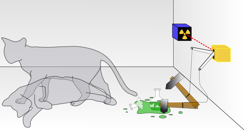
Schroedinger's Cat thought experiment is an extreme example of applying quantum mechanics to macroscopic objects, where naive quantum mechanics interpretation appears to contradict common sense.

Schrödinger's Cat: A cat, a flask of poison and a radioactive source are placed in a sealed box. If an internal monitor detects radioactivity, the flask is shattered, releasing the poison that kills the cat. The Copenhagen interpretation of quantum mechanics implies that after a while, the cat is simultaneously alive and dead. Yet, when we look in the box, we see the cat either alive or dead, not both alive and dead.

The textbook interpretation ( Copenhagen interpretation ) says, the cat+radioactive source is in an entangled state until one opens the box (measurement):
\[
\left.| \text{system} \right> = \frac{1}{\sqrt{2}} \left( \left.| : ) \right> \left.| 0 \right> + \left.| :( \right> \left.| 1 \right> \right)
\]
Entanglement implies the cat is both alive and dead before the box opened. But the application of quantum entanglement to a macro object, here cat, is controversial. In fact, the purpose of Schroedinger is to illustrate that quantum state (eps. wavefunction) may not be legitimate for describe macro system.

It's undoubted that there is something we don't know in the box, due to the quantum nature of radioactivity. But lack of information should be distinguished from quantum uncertainty.  In the sense of classical information theory, Schrodinger's cat is merely a normal cat. It's in some definite state (alive or dead). Yet different observers have different information: the experimenter said I don't know; while the flea on the back of the cat (or the cat itself) clearly knows what happened. There are many things in this world we don't know. A lot of them are associated with some quantum mechanical object (such as atoms emitting light). But we don't say, they are entangled.

It might be possible some day, the classical uncertainly and the quantum uncertainly are unified in a weird way, just like many other interpretation of quantum mechanics hoped. But in Schroedinger's Cat experiment, they are different. The main point is that the classical uncertainty is artificial. The cat is a macro object, meaning that it has huge amount of particle exchange with the environment. Outside the box, we can hear for example its scratch  sound. It's possible that the sound wave is overwhelmed by the noise, or our ears are not good enough. In either case, there exists a threshold $E_c$. Let's assume the cat-poison-radioactivity can be treated in a quantum mechanical way (See the Feynman diagram below). We can calculate the amplitudes $\mathcal{T}_{fi}$.

Notice that the cat must have interaction with the environment, we must also include such diagrams:

The sound etc. made by the cat is  characterized by $E$, $E_c$ is the threshold of the detector. 

The correction has similar structure with QED soft bremsstrahlung. In fact, we can assume the interaction of cat via environment is via QED ( for example, we can put a charge on the cat, and detect the electric field stirring outside the box). Let's simply borrow QED soft bremsstrahlung correction formula:
\[
 T'_{fi} = T^{(0)}_{fi} \cdot \exp\{ - f ( E / E_c) \}
\]
where $f(x)$ is increasing function.

The meaning of the result is, for a macro object, the correction always exist. In the case of an infinitely accurate detector, the classical cat and quantum cat cannot be distinguished by experiment. However, the amplitude is zero, i.e. still we can distinguish the classical cat and the quantum cat.

Dynamics of Undirected Graphs

It's understandable that each undirected graph is also a two-body interaction system. Because we can take its adjacency matrix or Laplacian matrix, which is the adjacency matrix but the diagonal terms are filled with degrees, as the Hamiltonian. Let's take a look at an example, path graph P2.

Fig. 1, P2

It's adjacency matrix can be written as: \[
H=\left(
\begin{array}{c c}
0 & 1 \\
1 & 0
\end{array} \right)
\]
As a physics student, the first thing I want to do is diagonalizing the Hamiltonian and solving for eigenspectrum.

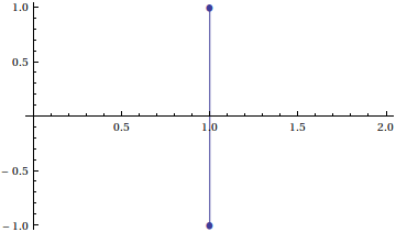
Let's do it. Obviously $H$ has two eigenvalues, $\pm 1$. The corresponding eigenvector are $(1, 1), (1, -1)$. Wait, what does it mean by a vector like $(1, -1)$? We know that $( 1, 0)$ can be used to represent the fist vertex $v_1$, and $(0, 1)$ the second, $v_2$. This is a puzzle. Especially for arbitrary undirected graph, the eigenvalues are reals. Not to mention directed graphs!

I found a nice idea from Dr. Dan Spielman's lecture [1]. He argues that these reals can be used as coordinates of the vertices. For our simplest example, vector $(1, -1)$ indicates the coordinates for $v_1, v_2$ are 1, -1. Of course we can pick two eigenvectors and therefore get two dimensional coordinates $v_1 : ( 1, 1), v_2 (1, -1)$. It can be shown below in Fig. 2. This geometric representation of graphs is called eigenvector projection.

Fig. 2, P2 in eigenvector space.

Let's play around for some slightly more complicated graphs. I'll start with a ring $C_{20}$.

Fig. 3, $C_{20}$

Instead of using adjacency matrix, Laplacian matrix is used, which is defined as: \[
L_{i j} = \left\{ \begin{array}{cc}
\text{deg}(i) \qquad i = j; \\
- a_{i, j} \qquad i \ne j;\\
\end{array} \right.
\] where $a_{i,j}$ is the entry of adjacency matrix. The Laplacian matrix of an undirected unweighted graph has the following property:

1. It is positive defined. 
2. It always has an eigenvector $(1, 1, \cdots 1)$, the corresponding eigenvalue is 0. 
3. The multiplicity $p$ of eigenvalue 0, is the number of connected components of the graph. 
4. Further more, the second second smallest eigenvalue of Laplacian matrix is called the algebraic connectivity. It is a characteristic parameter of the connectivity of the graph.

Fig. 4. Eigen-projection of $C_{20}$, use the 1st and 2nd eigenvectors. (sorted by eigenvalues)

Fig. 5, 1 - 3rd eigenvectors of $C_{20}$. (sorted by eigenvalues)

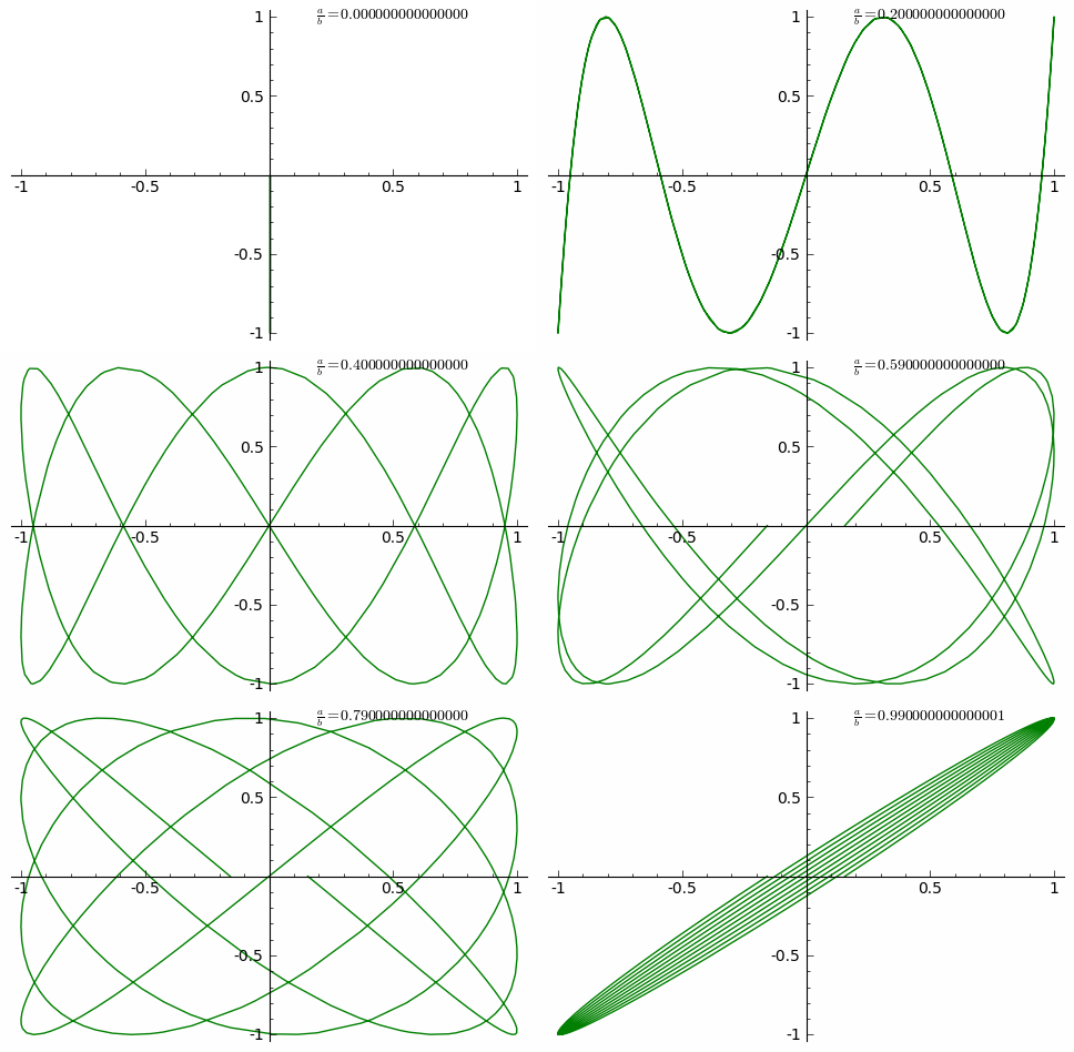
From Fig. 5, we can see harmonic modes that we are familiar with in physics. So besides the mathematical argument, we also have visualization of eigenvectors from the point of view of physics, as you expect. These eigenvalues are just the energy spectrum, with eigenvectors of the modes. The (2 dimensional) eigen-projections of a graph, therefore is the what we call Lissajous curves.

Fig. 6 Lissajous curves of various pair of modes.

The Lissajous curves of harmonics may have some aesthetic  value. Yet for discrete object like graphs, only the low energy modes generate smooth Lissajous curves. The high frequency modes are known as "fuzzy" ones.

Fig. 8 Eigen-projection of $C_{20}$ by the 2nd and 4th modes.

The eigenvector projection goes to crazy when the graphs get complicated. Several examples are presented below.

Fig. 9, A graph $C_{50}(7)$.

Fig. 12 Projection on the last two eigenvectors.

It can be shown, in the space spanned by the full eigenvectors, this projection provides an optimal graph layout under several constraints. For example, the eigenvector projection minimizes the following function:

\[
   z = \sum_{v_i, v_j \in V} A_{i,j} d^{(p)}_{i,j}
 \]
with subjected to the constraint: \[ \sum_{v_i, v_j \in V} d^{(p)}_{i,j} = 1.\], where $d^{(p)}$ is $p$ dimensional distance.

Unfortunately, it is difficult to directly visualize system in high dimensions. In 3 dimension or 2 dimension, the eigenvector projection tends to  squeeze in some directions, therefore not preferred for display small graphs.

In physics, the Hamiltonian matrix is always given in some basis, for instance quantum mechanical version of real space (Hilbert space). It is difficult to plant Hilbert space on a graph, yet nature has provided us a vector space on vertices, the tangent bundle $TG$, or the space of small vibrations, in the perspective of physics. We can take the $L^2$ space associated with this space as Hilbert space.

Therefore, the eigenvectors and eigenvalues can be seen as the modes of small vibrations of the graph instead of the actual position of graph vertices . Eigenvalues, as you wish, are just frequencies, or energies. The vibration picture allows us to make use of the full information of the eigensystem. I produced some animations of some vibrating graphs. Well, yeah, these are not so pretty... I'll try to make some better ones.

dim = 5;
lapmat = Table[If[i == j, dim - 1, -1], {i, 1, dim}, {j, 1, dim}];
MatrixForm[lapmat]

g0 = GraphPlot3D[lapmat, 
  VertexRenderingFunction -> ({Orange, Opacity[0.9], 
      Sphere[#1, .08]} &), 
  EdgeRenderingFunction -> ({ColorData["TemperatureMap", 0.2], Thick, 
      Opacity[0.7], Line[#1]} &), Method -> Automatic, 
  PlotStyle -> Directive[PointSize[0.05]], Boxed -> False, 
  ImageSize -> 400, BoxRatios -> {1, 1, 1}]

coor = VertexCoordinateRules /. Cases[g0, _Rule, Infinity];
{eval, evec} = Eigensystem[lapmat];

Manipulate[
 GraphPlot3D[lapmat, PlotStyle -> Thick, 
  VertexRenderingFunction -> ({Orange, Opacity[0.9], 
      Sphere[#1, .08]} &), 
  EdgeRenderingFunction -> ({ColorData["TemperatureMap", 0.2], Thick, 
      Opacity[0.7], Line[#1]} &), Boxed -> False,
  VertexCoordinateRules -> 
   Table[i -> (coor[[i]] + 
       amp*Sin[eval[[n]] t]*{evec[[i, x]], evec[[i, y]], 
         evec[[i, x]]}), {i, 1, dim}] , ViewPoint -> {10, 2, 0.4}, 
  BoxRatios -> {1, 1, 1}], {t, 0, 2 Pi}, {x, 1, dim, 1}, {y, 1, dim, 
  1}, {z, 1, dim, 1}, {{amp, 0.03}, 0, 0.1}, {n, 1, dim, 1}]

Fig. 15, one of the vibration modes of K4

Fig. 16, one of the vibration mode of K4

Fig. 17, one of the vibration mode of K4

Fig. 18, vibration modes of a string graph.

Update (Dec. 4, 2011):

This provides a simplest "quantum field" model. One may view the lattice graph as the timespace lattice (with respect to some basis). Of course, the discrete model has significant differences from continuous ones. Therefore, only the low energy modes can be used.

Mathematical interests on these vibrating graphs arises when these is a (finite) group, usually the symmetry group of the graph, acting on it (Consider the complete graph $K_4$. The Hilbert space we planted on the graph serves as the linear representations of the group. Therefore, certain eigenvectors may be orthogonal by group theory. In physics, the square of Hermitian inner product of vectors are proportion to transition probability. It can be observed through atomic spectra distribution and intensity. Therefore, the group representations determine the atomic spectra. This is another story behind the vibration of graphs. Although I'm in physics, I learned it from one of my math teachers, Dr. Basak Tathagata. The details are beyond my capability. E. Wigner's book is canonical on this subject.

Update (Jan. 7, 2012)
Significant change has been made. I used Laplacian matrix this time. It yields positive, well ordered eigenspectrum. Therefore, almost all graphs were updated. I still use Mathematica to generate graphs. But a software gifsicle was used to generate animations gif picture. Mirage serves as gif viewer.