It's understandable that each undirected graph is also a two-body interaction system. Because we can take its adjacency matrix or Laplacian matrix, which is the adjacency matrix but the diagonal terms are filled with degrees, as the Hamiltonian.
Let's take a look at an example, path graph P2.
It's adjacency matrix can be written as: \[
H=\left(
\begin{array}{c c}
0 & 1 \\
1 & 0
\end{array} \right)
\]
As a physics student, the first thing I want to do is diagonalizing the Hamiltonian and solving for eigenspectrum.
Let's do it. Obviously $H$ has two eigenvalues, $\pm 1$. The corresponding eigenvector are $(1, 1), (1, -1)$. Wait, what does it mean by a vector like $(1, -1)$? We know that $( 1, 0)$ can be used to represent the fist vertex $v_1$, and $(0, 1)$ the second, $v_2$. This is a puzzle. Especially for arbitrary undirected graph, the eigenvalues are reals. Not to mention directed graphs!
I found a nice idea from Dr. Dan Spielman's lecture [1]. He argues that these reals can be used as coordinates of the vertices. For our simplest example, vector $(1, -1)$ indicates the coordinates for $v_1, v_2$ are 1, -1. Of course we can pick two eigenvectors and therefore get two dimensional coordinates $v_1 : ( 1, 1), v_2 (1, -1)$. It can be shown below in Fig. 2. This geometric representation of graphs is called eigenvector projection.
Let's play around for some slightly more complicated graphs. I'll start with a ring $C_{20}$.
Instead of using adjacency matrix, Laplacian matrix is used, which is defined as: \[
L_{i j} = \left\{ \begin{array}{cc}
\text{deg}(i) \qquad i = j; \\
- a_{i, j} \qquad i \ne j;\\
\end{array} \right.
\] where $a_{i,j}$ is the entry of adjacency matrix. The Laplacian matrix of an undirected unweighted graph has the following property:
From Fig. 5, we can see harmonic modes that we are familiar with in physics. So besides the mathematical argument, we also have visualization of eigenvectors from the point of view of physics, as you expect. These eigenvalues are just the energy spectrum, with eigenvectors of the modes. The (2 dimensional) eigen-projections of a graph, therefore is the what we call Lissajous curves.
The Lissajous curves of harmonics may have some aesthetic value. Yet for discrete object like graphs, only the low energy modes generate smooth Lissajous curves. The high frequency modes are known as "fuzzy" ones.
The eigenvector projection goes to crazy when the graphs get complicated. Several examples are presented below.
It can be shown, in the space spanned by the full eigenvectors, this projection provides an optimal graph layout under several constraints. For example, the eigenvector projection minimizes the following function:
\[
z = \sum_{v_i, v_j \in V} A_{i,j} d^{(p)}_{i,j}
\]
with subjected to the constraint: \[ \sum_{v_i, v_j \in V} d^{(p)}_{i,j} = 1.\], where $d^{(p)}$ is $p$ dimensional distance.
Unfortunately, it is difficult to directly visualize system in high dimensions. In 3 dimension or 2 dimension, the eigenvector projection tends to squeeze in some directions, therefore not preferred for display small graphs.
In physics, the Hamiltonian matrix is always given in some basis, for instance quantum mechanical version of real space (Hilbert space). It is difficult to plant Hilbert space on a graph, yet nature has provided us a vector space on vertices, the tangent bundle $TG$, or the space of small vibrations, in the perspective of physics. We can take the $L^2$ space associated with this space as Hilbert space.
Therefore, the eigenvectors and eigenvalues can be seen as the modes of small vibrations of the graph instead of the actual position of graph vertices . Eigenvalues, as you wish, are just frequencies, or energies. The vibration picture allows us to make use of the full information of the eigensystem. I produced some animations of some vibrating graphs. Well, yeah, these are not so pretty... I'll try to make some better ones.
Update (Dec. 4, 2011):
This provides a simplest "quantum field" model. One may view the lattice graph as the timespace lattice (with respect to some basis). Of course, the discrete model has significant differences from continuous ones. Therefore, only the low energy modes can be used.
Mathematical interests on these vibrating graphs arises when these is a (finite) group, usually the symmetry group of the graph, acting on it (Consider the complete graph $K_4$. The Hilbert space we planted on the graph serves as the linear representations of the group. Therefore, certain eigenvectors may be orthogonal by group theory. In physics, the square of Hermitian inner product of vectors are proportion to transition probability. It can be observed through atomic spectra distribution and intensity. Therefore, the group representations determine the atomic spectra. This is another story behind the vibration of graphs. Although I'm in physics, I learned it from one of my math teachers, Dr. Basak Tathagata. The details are beyond my capability. E. Wigner's book is canonical on this subject.
Update (Jan. 7, 2012)
Significant change has been made. I used Laplacian matrix this time. It yields positive, well ordered eigenspectrum. Therefore, almost all graphs were updated. I still use Mathematica to generate graphs. But a software gifsicle was used to generate animations gif picture. Mirage serves as gif viewer.
 |
| Fig. 1, P2 |
H=\left(
\begin{array}{c c}
0 & 1 \\
1 & 0
\end{array} \right)
\]
As a physics student, the first thing I want to do is diagonalizing the Hamiltonian and solving for eigenspectrum.
Let's do it. Obviously $H$ has two eigenvalues, $\pm 1$. The corresponding eigenvector are $(1, 1), (1, -1)$. Wait, what does it mean by a vector like $(1, -1)$? We know that $( 1, 0)$ can be used to represent the fist vertex $v_1$, and $(0, 1)$ the second, $v_2$. This is a puzzle. Especially for arbitrary undirected graph, the eigenvalues are reals. Not to mention directed graphs!
I found a nice idea from Dr. Dan Spielman's lecture [1]. He argues that these reals can be used as coordinates of the vertices. For our simplest example, vector $(1, -1)$ indicates the coordinates for $v_1, v_2$ are 1, -1. Of course we can pick two eigenvectors and therefore get two dimensional coordinates $v_1 : ( 1, 1), v_2 (1, -1)$. It can be shown below in Fig. 2. This geometric representation of graphs is called eigenvector projection.
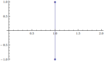 |
| Fig. 2, P2 in eigenvector space. |
Let's play around for some slightly more complicated graphs. I'll start with a ring $C_{20}$.
 |
| Fig. 3, $C_{20}$ |
Instead of using adjacency matrix, Laplacian matrix is used, which is defined as: \[
L_{i j} = \left\{ \begin{array}{cc}
\text{deg}(i) \qquad i = j; \\
- a_{i, j} \qquad i \ne j;\\
\end{array} \right.
\] where $a_{i,j}$ is the entry of adjacency matrix. The Laplacian matrix of an undirected unweighted graph has the following property:
- It is positive defined.
- It always has an eigenvector $(1, 1, \cdots 1)$, the corresponding eigenvalue is 0.
- The multiplicity $p$ of eigenvalue 0, is the number of connected components of the graph.
- Further more, the second second smallest eigenvalue of Laplacian matrix is called the algebraic connectivity. It is a characteristic parameter of the connectivity of the graph.
 |
| Fig. 4. Eigen-projection of $C_{20}$, use the 1st and 2nd eigenvectors. (sorted by eigenvalues) |
 |
| Fig. 5, 1 - 3rd eigenvectors of $C_{20}$. (sorted by eigenvalues) |
From Fig. 5, we can see harmonic modes that we are familiar with in physics. So besides the mathematical argument, we also have visualization of eigenvectors from the point of view of physics, as you expect. These eigenvalues are just the energy spectrum, with eigenvectors of the modes. The (2 dimensional) eigen-projections of a graph, therefore is the what we call Lissajous curves.
 |
| Fig. 6 Lissajous curves of various pair of modes. |
The Lissajous curves of harmonics may have some aesthetic value. Yet for discrete object like graphs, only the low energy modes generate smooth Lissajous curves. The high frequency modes are known as "fuzzy" ones.
 |
| Fig. 8 Eigen-projection of $C_{20}$ by the 2nd and 4th modes. |
 |
| Fig. 9, A graph $C_{50}(7)$. |
 |
| Fig. 12 Projection on the last two eigenvectors. |
It can be shown, in the space spanned by the full eigenvectors, this projection provides an optimal graph layout under several constraints. For example, the eigenvector projection minimizes the following function:
\[
z = \sum_{v_i, v_j \in V} A_{i,j} d^{(p)}_{i,j}
\]
with subjected to the constraint: \[ \sum_{v_i, v_j \in V} d^{(p)}_{i,j} = 1.\], where $d^{(p)}$ is $p$ dimensional distance.
Unfortunately, it is difficult to directly visualize system in high dimensions. In 3 dimension or 2 dimension, the eigenvector projection tends to squeeze in some directions, therefore not preferred for display small graphs.
In physics, the Hamiltonian matrix is always given in some basis, for instance quantum mechanical version of real space (Hilbert space). It is difficult to plant Hilbert space on a graph, yet nature has provided us a vector space on vertices, the tangent bundle $TG$, or the space of small vibrations, in the perspective of physics. We can take the $L^2$ space associated with this space as Hilbert space.
Therefore, the eigenvectors and eigenvalues can be seen as the modes of small vibrations of the graph instead of the actual position of graph vertices . Eigenvalues, as you wish, are just frequencies, or energies. The vibration picture allows us to make use of the full information of the eigensystem. I produced some animations of some vibrating graphs. Well, yeah, these are not so pretty... I'll try to make some better ones.
dim = 5;
lapmat = Table[If[i == j, dim - 1, -1], {i, 1, dim}, {j, 1, dim}];
MatrixForm[lapmat]

g0 = GraphPlot3D[lapmat,
  VertexRenderingFunction -> ({Orange, Opacity[0.9],
      Sphere[#1, .08]} &),
  EdgeRenderingFunction -> ({ColorData["TemperatureMap", 0.2], Thick,
      Opacity[0.7], Line[#1]} &), Method -> Automatic,
  PlotStyle -> Directive[PointSize[0.05]], Boxed -> False,
  ImageSize -> 400, BoxRatios -> {1, 1, 1}]

coor = VertexCoordinateRules /. Cases[g0, _Rule, Infinity];
{eval, evec} = Eigensystem[lapmat];

Manipulate[
 GraphPlot3D[lapmat, PlotStyle -> Thick,
  VertexRenderingFunction -> ({Orange, Opacity[0.9],
      Sphere[#1, .08]} &),
  EdgeRenderingFunction -> ({ColorData["TemperatureMap", 0.2], Thick,
      Opacity[0.7], Line[#1]} &), Boxed -> False,
  VertexCoordinateRules ->
   Table[i -> (coor[[i]] +
       amp*Sin[eval[[n]] t]*{evec[[i, x]], evec[[i, y]],
         evec[[i, x]]}), {i, 1, dim}] , ViewPoint -> {10, 2, 0.4},
  BoxRatios -> {1, 1, 1}], {t, 0, 2 Pi}, {x, 1, dim, 1}, {y, 1, dim,
  1}, {z, 1, dim, 1}, {{amp, 0.03}, 0, 0.1}, {n, 1, dim, 1}]
 |
| Fig. 15, one of the vibration modes of K4 |
 |
| Fig. 16, one of the vibration mode of K4 |
 |
| Fig. 17, one of the vibration mode of K4 |
 |
| Fig. 18, vibration modes of a string graph. |
Update (Dec. 4, 2011):
This provides a simplest "quantum field" model. One may view the lattice graph as the timespace lattice (with respect to some basis). Of course, the discrete model has significant differences from continuous ones. Therefore, only the low energy modes can be used.
Mathematical interests on these vibrating graphs arises when these is a (finite) group, usually the symmetry group of the graph, acting on it (Consider the complete graph $K_4$. The Hilbert space we planted on the graph serves as the linear representations of the group. Therefore, certain eigenvectors may be orthogonal by group theory. In physics, the square of Hermitian inner product of vectors are proportion to transition probability. It can be observed through atomic spectra distribution and intensity. Therefore, the group representations determine the atomic spectra. This is another story behind the vibration of graphs. Although I'm in physics, I learned it from one of my math teachers, Dr. Basak Tathagata. The details are beyond my capability. E. Wigner's book is canonical on this subject.
Update (Jan. 7, 2012)
Significant change has been made. I used Laplacian matrix this time. It yields positive, well ordered eigenspectrum. Therefore, almost all graphs were updated. I still use Mathematica to generate graphs. But a software gifsicle was used to generate animations gif picture. Mirage serves as gif viewer.
impressive
ReplyDelete