Symmetry factor is a well-known easy-to-confuse factor for beginners of quantum field theory (QFT). Although most textbooks give rules or even list symmetry factors of Feynman diagrams up to an order that non-experts perhaps would never have a chance to compute (See for example [1-6]). It is not satisfactory for me, because these treatments either show tedious but ambiguous instructions [2-6] which is scary and confusing, or sketch some abstract theorem, in which case one have to check other references for practical instructions [1]. There are also informal but nice discussions on some Q&A websites such as
MathOverflow, StackExchange [7]. A formal definition and a set of reliable rules as far as I know still lack. This article is intended to provide such a description. The main idea is abstracted from the references mentioned above.
1.
Symmetry Factor as a Factor of Symmetry
Symmetry factor arises from counting Feynman diagrams. Generally, the symmetry factor $\text{Sym}(f)$ of a Feynman diagram $f$ is the order (size) of its
automorphism group $\text{Aut}(f)$ [1,7], namely, \[ \text{Sym}(f) \equiv \text{Aut}(f). \] $\text{Aut}(f)$ is the
symmetry group of the Feynman diagram $f$, which is implied the name of symmetry factor. The benefit of this idea is that the automorphism group is clearly defined, once the Feynman diagram is specified.
For example, Feynman diagram \[ f = \int \mathrm{d}^4 x_0 \mathrm{d}^4 x_1 \mathrm{d}^4 x_2 \mathrm{d}^4 x_3 J(x_1) D(x_1 - x_0) J(x_2) D(x_2 - x_0) J(x_3) D(x_3 - x_0) \] appearing in Path Integral of scalar $\varphi^3$ theory , can be "represented" by a star graph $S_3$ (Fig. 1). Whereas, $\text{Aut}(S_3) = D_6$, is the dihedral group of order 6, indicating $\text{Sym}(f) = 6$.
 |
| Fig. 1, a star graph $S_3$. |
Feynman diagrams may arise from different contexts, yet the symmetry factor always exits, being equal or related. In order to treat Feynman diagrams systematically, we require some generic information of Feynman diagrams. The collection of diagrams, of course, must be known. We also need to know how to compare the "structure" of different Feynman diagrams. This is specified by isomorphisms defined among Feynman diagrams. In addition, quantum superposition implies that any physical observable could not distinguish coherent states that represented by "structurally the same" Feynman diagrams, hence would equally include "structurally the same" diagrams.
An isomorphism is a bijective structure-preserving map $\beta: x \to y$ between Feynman diagrams $x$ and $y$. The meaning of structure-preserving should be specified by the theory, namely the definition of Feynman diagrams. Roughly speaking, structure-preserving map gives the same Feynman diagram up to some labels. An automorphism of a Feynman diagram $x$ is an isomorphism that maps $x$ to itself. All automorphisms form a group under composition, denoted by $\text{Aut}(x)$.
Let $\mathcal{F} = (\text{Ob}(\mathcal{F}), \text{Iso}(\mathcal{F}) )$ be an ordered pair, where
- $\text{Ob}(\mathcal{F})$ is a set of Feynman diagrams;
- $\text{Iso}(\mathcal{F})$ is a set of Isomorphisms of Feynman diagrams;
- $t: \text{Iso}(\mathcal{F}) \to \text{Ob}(\mathcal{F})$ assigns a Feynman diagram to each isomorphism, called target;
- $s: \text{Iso}(\mathcal{F}) \to \text{Ob}(\mathcal{F})$ assigns a Feynman diagram to each isomorphism, called source;
together with
- a $\mathbb{C}$-linear structure $\sharp$ on $\text{Ob}(\mathcal{F})$, namely $\text{Ob}(\mathcal{F})$ forms a vector space $\mathbb{C}[\text{Ob}(\mathcal{F})] \equiv \mathbb{C}[\mathcal{F}]$;
- a linear map $\mathcal{A}: \mathbb{C}[\mathcal{F}] \to \mathbb{C}$.
The linear structure on $\text{Ob}(\mathcal{F})$ comes from the principle of quantum superposition. A process is a superposition of various Feynman diagrams. The linear map $\mathcal{A}$ evaluates the amplitude of a series of Feynman diagrams. We require that $\beta \circ \mathcal{A} = \mathcal{A} \circ \beta$ for all isomorphisms $\beta$. It means that, if two Feynman diagrams have the same structure, their amplitudes are equal. Sometimes, a known phase factor is allowed, such as in fermion field. It will be discussed later.
$\mathcal{F}$ generally should be given by the theory which defines the Feynman diagrams. Notice that $\mathcal{F}$ forms a groupoid (category theory).
Pick $x \in \text{Ob}(\mathcal{F})$ and denote $s^{-1}(x) = \{ \alpha \in \text{Iso}(\mathcal{F}) | \alpha : x \to y, \forall y \in \text{Ob}(\mathcal{F}) \}$. An orbit of $x$ is defined as the set $\mathcal{O}_x = \{ \beta \cdot x | \beta \in s^{-1}(x) \}$. It collects all structurally the same diagrams.
Any physical quantum process is a function of orbits, namely, if a physical quantum process consists one Feynman diagram $x$, it contains the whole orbit of $x$ . The set of orbit is denoted as $\mathfrak{O} = \text{Ob}(\mathcal{F})/\text{Iso}(\mathcal{F}) = \{ \mathcal{O}_x | x \in \text{Ob}(\mathcal{F}) \}$. Let $q$ be such a quantum process,\[
q = \sum_{x \in X} c_{\mathcal{O}_x} \cdot x \qquad (c_{\mathcal{O}_x} \in \mathbb{C})
\]The sum can be rewritten over orbits:\[
q = \sum_{ \mathcal{O} \in \mathfrak{O}} c_{\mathcal{O}} \cdot \sum_{x \in \mathcal{O}} x
\] Therefore, amplitude of the process \[
\mathcal{A}(q) = \sum_{ \mathcal{O} \in \mathfrak{O}} c_{\mathcal{O}} \cdot \sum_{x \in \mathcal{O}} \mathcal{A}(x) = \sum_{ \mathcal{O} \in \mathfrak{O}} c_{\mathcal{O}} \cdot |\mathcal{O}| \cdot \mathcal{A}(\mathcal{O})
\]
Lemma: $|\mathcal{O}_x| = | s^{-1}(x)| / |\text{Aut}(x)|$.
Proof: define a map $\phi: s^{-1}(x) \to \mathcal{O}_x$ by $ \alpha \mapsto \alpha \cdot x$. This map is surjective by definition of $\mathcal{O}_x$.
$\forall \alpha, \beta \in s^{-1}(x), \alpha \cdot x = \beta \cdot x \implies \alpha \beta^{-1} \cdot x = x \implies \alpha \beta^{-1} \in \text{Aut}(x)$.
Therefore, $\alpha \equiv \beta \mod \text{Aut}(x) $. By the
quotient theorem for surjections, there exits a bijection $\zeta: s^{-1}(x)/\text{Aut}(x) \to \mathcal{O}_x$. Hence, $|\mathcal{O}_x| = | s^{-1}(x) / \text{Aut}(x)|$.
Moreover, $\text{Aut}(x)$ partitions $s^{-1}(x)$. $\forall \alpha, \beta \in s^{-1}(x), \alpha \cdot \text{Aut}(x), \beta \cdot \text{Aut}(x)$ are two equivalence classes. There exits a bijection $ \xi = \beta \circ \alpha^{-1} $ between them. So $|\alpha \cdot \text{Aut}(x)| = |\beta \cdot \text{Aut}(x)| \implies | s^{-1}(x) / \text{Aut}(x)| = | s^{-1}(x) | / | \text{Aut}(x)| \qquad \blacksquare$.
If there exits a group $G$ and a group action $\lambda: G \to \text{Iso}(\mathcal{F})$ such that 1. $\lambda$ is surjective 2. $\lambda(g \cdot h)(x) = \lambda(g) \circ \lambda(h) (x) \quad \forall g, h \in G, x \in \text{Ob}(\mathcal{F})$, then
orbit-stabilizer theorem applies. $|\mathcal{O}_x| = | G |/|G_x|$. $\lambda$ induces a surjective group homomorphism from $G_x$ to $\text{Aut}(x)$. The First Isomorphism Theorem implies $G_x / \text{Ker} \lambda = \text{Aut}(x)$. Hence $|\mathcal{O}_x| = |G| / |\text{Ker}\lambda| \cdot 1/|\text{Aut}(x)| $.
In either case, $\text{Aut}(x)$ appears in the denominator: \[ \mathcal{A}(q) = \sum_{\mathcal{O} \in \mathfrak{O} } F(\mathcal{O}) \frac{ c_{\mathcal{O}}}{ |\text{Aut}(\mathcal{O})| } \mathcal{A}(\mathcal{O}) \]. Note that $\text{Aut}(x) = \text{Aut}(y)$ if $x, y$ are in the same orbit. Factor $F(\mathcal{O})$ is always easier to compute: it is usually a function of number of vertices and number of propagators of a Feynman diagram. And therefore often canceled by pre-defined factors. The rewritten expression only sum over structurally distinct Feynman diagrams. $ \text{Aut}(\mathcal{O}) $ therefore serves as symmetry factor. If the pre-defined factors, $s^{-1}(x)$ or $|G|/|\text{Ker} \lambda|$ are not well coordinated, some common factor may enter the symmetry factor, which complicates the case. We assume here, the theory is defined cleverly, so that we don't have to worry about it.
Sometimes, the amplitudes of two isomorphic diagrams may differ by a known scalar factor, similar derivation applies: \[
\mathcal{A}(q) = \sum_{\mathcal{O} \in \mathfrak{O}} \frac{c_{\mathcal{O}} }{|\text{Aut}(\mathcal{O})|} \cdot \left( \sum_{\beta \in s^{-1}(x_\mathcal{O})} \theta( \beta \cdot \text{Aut}(\mathcal{O})) \right ) \mathcal{A}(\mathcal{O}) . \]
In fermion cases, the propagators are grassmannian. Any transposition of propagators results a $-1$ factor. If $\text{Aut}(x)$ of a Feynman diagram $x$ consists nontrivial permutation of propagators, $x$ can always find a propagator transposition partner that is exactly itself. Hence its amplitude must vanish. Therefore, the symmetry factor for fermion lines is always trivial.
2. Feynman Diagram as a Graph
In above discussion, we did not specify Feynman diagrams, only requiring some general algebraic structures. Knowing the specific structure of Feynman diagrams is always the first step for practical calculations. It turns out, that in most cases, Feynman diagrams are
colored (labeled) graphs that allow mixed edges (directed, undirected), multi-edges and loops $\S$.
Definition of graphs[10]:
A graph is an ordered triplet $g = (V, A, t)$, where
- $V$ is a set, its elements are called vertices $\ddagger$;
- $A$ is a set, its elements are called arcs;
- $t: A \to V \times V$ is a map, assigning to each arc a partial ordered pair of vertices, called source and target.
Undirected graphs can be defined in the same way but using unordered pair of vertices. A graph isomorphism $\lambda: g \to g'$ between graph $g=(V, A, t)$ and $g' = (V', A', t')$ is a pair of maps $\lambda = (\nu, \alpha), \nu: V \to V', \alpha: A \to A'$ preserving the graph connectivity. Namely, the following diagram commutes:
An automorphism of a graph is a bijective isomorphism to itself. All graphs form a category $\mathcal{G}$. Feynman diagrams of a theory can be represented by graphs (called Feynman graphs). A graph representation of Feynman diagrams $\mathcal{F}$ is a
functor $F: \mathcal{F} \to \mathcal{G}$. Symmetry factor of a Feynman diagram is precisely the order of automorphism group of its Feynman graph, if the graph representation is faithful, i.e. one-to-one.
The graph representation of Feynman diagrams immediately leads to the following reduction theorem:
Lemma [12]:
Let $A, H$ be finite groups, $\Omega$ finite set. $H$ acts on $\Omega$.
\[
\left| A \wr_\Omega H \right| = \left| A \right|^{\left| \Omega \right|} \left| H \right|
\], where $\wr$ is the wreath product. If $\Omega = \{1, 2, ... n\}$, $H = S_n$ acting on $\Omega$ by permutation, $A \wr_\Omega S_n $ can be written as $A \wr S_n$ for simplicity.
Theorem [11] :
Let $g_1, g_2, \cdots g_k$ be pairwise non-isomorphic connected graphs and $g$ is the disjoint union of $m_i$ copies of $g_i, i = 1, \cdots, k$. Then
\[
\text{Aut}(g) = \text{Aut}(g_1) \wr S_{m_1} \times \cdots \times \text{Aut}(g_k) \wr S_{m_k},
\]\[
| \text{Aut}(g) | = | \text{Aut}(g_1)|^{m_1} m_1! \times \cdots \times |\text{Aut}(g_k)|^{m_k} m_k!
\]
In the language of physics,
the symmetry factor of a Feynman diagram equals the product of symmetry factors of its disconnected components times the order of symmetry group of the set of subgraphs. This well-known result allows us to reduce the calculation of symmetry factors into irreducible diagrams.
This graphical representation can be used directly for computing Feynman diagrams of small size. Consider a vacuum bubble shown by Fig. 1 from some scalar $\varphi^3$ theory. An undirected graph is enough to represent it. 3! permutations of edges and 2 permutations of vertices map the graph to itself. This gives the symmetry factor $2 \times 3!$.
 |
| Fig. 2 Vacuum Bubble. Symmetry factor = $2 \times 3!$ |
For slightly complicated graphs, it is valuable to keep in mind that each automorphism consist two types of operation (either one could be identity) on a graph: permutation of vertices that does not cause the change arcs; permutation of arcs that does not cause the change of vertices.
The graph representation also bring convenience to counting the number of isomorphisms (the pre-factor). For example, for a graph $g$ with $V$ vertices, $E$ edges from some scalar theory, permutation of vertices is equivalent to relabeling of vertices, hence does not change the graph structure. The same goes to permutation of edges. Therefore, the number of graphs isomorphic to $g$ is $V! \cdot E!$.
For Feynman graphs from scalar theory, if the collection of Feynman graphs only consists diagrams having the same number of vertices $V$ and the same number of edges $E$, a group $G = S_V \cdot S_E$ can be used to induce the isomorphisms (see section 1).
Burnside's lemma: Let $X$ be finite set, and a finite group $G$ acts on it. Let $\mathcal{O}_x \equiv \{ g \cdot x | \forall g \in G \}$ be orbit, $X^g \equiv \{ x \in X | g\cdot x = x \}$ be elements fixed by $g \in G$, $X/G \equiv \{ \mathcal{O}_x | \forall x \in X \}$ be the set of orbit. Then \[
| X/G| = \frac{1}{|G|} \sum_{g \in G} | X^g|
\] Recall that topologically different Feynman diagrams belongs to different orbits. This gives a formula to count the number of topologically distinct Feynman graphs.
Counting permutations is not generally straightforward. 2D geometric symmetries (isometries, transformations that preserve the distances and angles) are more familiar to us. (Example Fig. 1) A simple graph is a graph without multi-edges or loops. It has been proven that any
undirected simple graph can be drawn on a plane such that each graph automorphism corresponds to a symmetry of the graphics on the plane [13-14]. Unfortunately, the algorithm of symmetric drawing of a general graph is highly non-trivial - it is a
NP-hard problem, at least as hard as determining the graph automorphism group. A general principle is that the edges should be drawn equal-lengthily, the non-edges should also be drawn equal-lengthily, where a non-edge is an imaginary line connecting two disconnected vertices.
A useful application is on planar graphs. A planar graph is a graph that can be drawn on a plane without edges crossing. If a planar graphs has a drawing that displays all the automorphisms, by the classification of 2D point groups, the 2D symmetry group hence the graph automorphism group is either cyclic group $C_n$ or dihedral group $D_{2n}$. It is worth mentioning Kuratowski's theorem that gives the sufficient and necessary condition of a planar graph.
Kuratowski's Theorem:
A graph $h$ is a minor of a graph $g$ if a copy of $h$ can be obtained from $g$ via repeated edge deletion and/or edge contraction. A graph is planar if and only if it contains neither $K_5$ or $K_{3,3}$ (Fig. 3 and 4) as graph minor.
Kuratowski's theorem provides a way to determine if a graph is planar. According to the theorem,
a graph with vertices less than 5, or edges less than 9 would always be planar. Notice that external lines and vertices does not contribute to the embedding. This fact further helps reduce the possibility of being non-planar.
 |
| Fig. 3 graph $K_5$ |
 |
| Fig. 4 graph $K_{3,3}$ |
 |
| Fig. 5 the first non-planar graph in $\varphi^3$ theory. It is actually $K_{3,3}$. |
The above discussion can be summarized as, draw a planar graph "nicely", and rotate it as many as possible and then do one reflection do find the symmetries, which is a subgroup of the graph automorphism group; if one is lucky enough, that is the graph automorphism group. In fact, if for every two vertices "looks equivalent", if there exits a transformation connecting them, the symmetry group is pretty much the automorphism group.
The symmetries between multi-edges are merely the permutations of the multi-edges. The symmetry factor of each loop is always 2 for scalar theory. Therefore, the contribution of multi-edges and loops to symmetry factor is easily added. Details will be explained later. Examples (See Fig. 6):
|
Fig. 6 examples (taken from [4]) |
a. Two loops give $2^2$, a double-edge gives $2$. The skeleton of the graph then is planar. A rotation of $\pi$ preserves it, hence has $C_2$ symmetry. $S = 2^2 \times 2 \times 2$
b. Loops and multi-edge give $2^2$. The skeleton adopts a reflection symmetry (with respect to horizontal line), hence has $D_2$ symmetry. $S = 2^2 \times 2$.
c. Multi-edge gives $2^2$. The skeleton is a rectangle (not square, because a single edge is still different from a multi-edge) in equilateral form. It adopts $D_4$ symmetry, generated by a rotation of $\pi$ and a reflection. $S = 2^2 \times 4$.
d. Loops give $2^3$. The rest is adopts $D_6$ symmetry. $2^3 \times 6$.
e. This graph is planar but not equilateral. In fact in 3D, it is a tetrahedron, adopting $T_3$ symmetry. Also, using the original definition of a graph, it allows all permutations of vertices regardless the alignment of vertices. Therefore $\text{Aut}(e) = S_4$. $S = 4!$.
3. Feynman diagrams beyond simple graphs: labeling, sources, multi-edges, loop and arc orientations
In section 1, we define Feynman diagrams as arbitrary objects that form a category. In section 2, we discussed the application of Feynman diagram in terms of Feynman graphs, especially undirected graphs, as they are usually thought to be. However, simple graph representation may not be faithful. More generally, Feynman diagrams come with decorations. Mathematically, they are called graph coloring or labeling. In this section, we discuss the possible decorations. If there is a coloring or any other decorations, the isomorphisms hence automorphisms should preserve the them. Therefore, some symmetries may be suppressed.
We now assume multi-edges, loop exit and arcs are directed. That is the usual case.
Multiple arcs over vertex $(v_1, v_2)$ is a set of arcs $t^{-1}(v_1, v_2) = \{ a \in A | t(a) = (v_1, v_2) \}$. If $|t^{-1}(v_1,v_2)| = 1$, it is called a single arc. Apparently, any permutation over $t^{-1}(v_1, v_2)$ preserves $t$ hence is an automorphism.
An arc $a \in t^{-1}(v_1, v_2)$ has an orientation, from $v_1$ to $v_2$. An orientation flip is a map $\tau: a \to a^{-1}$, where whenever $a \in t^{-1}(v_1, v_2)$, then $a^{-1} \in t^{-1}(v_2,v_1)$ (called an inverse of arc $a$), if both $a$ and $a^{-1}$ exist. Namely, arc $a^{-1}$ has opposite orientation to arc $a$. In a
scalar theory, each arc has an inverse ($|t^{-1}(v_1, v_2)| = |t^{-1}(v_2,v_1)|$ if multiple) and $\mathcal{A}( a ) = \mathcal{A}( a^{-1})$, i.e. the amplitudes are equal. Especially, arcs are defined by propagators, such as $D(x, y)$. Scalar theory simply requires that $D(x, y) \equiv D(y, x)$. So in a scalar theory orientation flips enter the isomorphisms. In fact, when arcs are directed,
neither transposition of two vertices like $\sigma: (v_1, v_2)$
nor orientation flip like $\tau: a \leftrightarrow a^{-1}$ preserves the graph. Instead, $\sigma \cdot \tau$ is always an automorphism. So we can incorporate orientation flips with vertices permutations and simply use undirected graphs as a representation. There is one exception, however, that is the loop. A loop $l$ is an arc with the target and source the same, $t(l) = (v, v)$. In this case, orientation must be defined separately. Orientation flip becomes an automorphism. Note that there is no vertex transposition between the same vertex, yet orientation flip always exits.
Therefore, in a scalar theory, each loop gives a symmetry factor of 2. In a
non-scalar theory, when orientation flip is not an isomorphism any more (i.e. $D(x,y) \ne D(y,x)$),
directed graph must be used, and loops does not gives a symmetry factor of 2 any more.
Feynman diagram vertices may be labeled by
sources. For example, a raw propagator in path integral formalism $\int d^4 x d^4 y d^4 z d^4 w \eta(x) D(x, y) D(y, z) D(y, z) D(z, w) \bar{\eta}(w)$ has two sources $\eta$ and $\bar \eta$. (See Fig xxx). Transposing a source and an other vertex certain does not preserve the diagram. Sources are labeled by dummy variables, thus in a scalar theory, their permutations are viewed as identity. One can simply think they are labeled by exacted the same label. One can even contract them into one vertex. Example of identical sources: from graphs on the right,
 |
| Fig. 7 left: Feynman diagrams with sources. right: sources contracted into a single one (black dot). |
a. Multi-edges gives $2^3$, the skeleton has a $D_{2}$ symmetry ( axial symmetry, reflection symmetry). $S = 2^3 \times 2$.
b. $D_{8}$ symmetry. $S = 8$.
c. Loops and multi-edges give $2^3$. the rest has a $D_2$ symmetry (one reflection). $S = 2^3 \times 2$.
d. Multi-edge gives $2$, and the rest only has a $D_2$ symmetry. $S = 2 \times 2$.
e. Multi-edges give $2^2$. The skeleton is asymmetric. $S = 2^2$.
f. Multi-edge and loops give $2^2$. The skeleton is asymmetric. $S = 2 ^ 2$.
Diagram vertices usually also have external vertices on them. Permutation of external labels does not serve as isomorphisms. So when external vertices are can be seen as
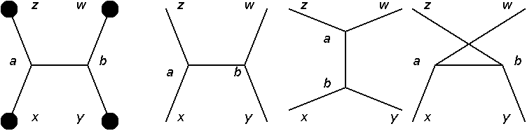
fixed by distinct labels. Automorphisms should also preserve these labels. For example, let $x_1, x_1$ be distinct vertices, $x$ an internal vertex, $a_1:(x_1, x), a_2:(x_2, x)$ two arcs. If $x_1, x_2$ are sources, $\tau: a_1 \leftrightarrow a_2$ is an automorphism. One can write down the path integral expression $\mathcal{W}[J] = \frac{1}{2} \int d^4x'_1 d^4 x'_2 d^4 x J(x'_1) D(x'_1 - x) J(x'_2) D(x'_2 - x)$. But when $x_1, x_2$ are labeled by external coordinates, i.e. by taking functional derivative to the $\mathcal{W}[J]$. The original automorphism $\tau: a_1 \leftrightarrow a_2$ does not preserve the label $x_1, x_2$, but does result to the same amplitude. Therefore $\tau$ is still an isomorphism yet not an automorphism. This non-automorphic isomorphism doubles the terms in $\mathcal{W}[J]$, which cancels the symmetry factor. One can check the pre-factor of the resulting expression. $\frac{\delta}{\delta J(x_1)}\frac{\delta}{\delta J(x_2)} \mathcal{W}[J]= \int d^4 x D(x_1 - x) D(x_2 - x)$. When propagators are fixed by 4-momentum, any isomorphism hence automorphism should also preserve these labels. (Example: Fig. 8)
 |
| Fig. 8 $t, s, u$ three channels generated by the same source diagram, but have to be considered separately, because of the labeling. |
Summary
- Reduce a Feynman diagram to several irreducible disconnected components. Symmetry factor of the large Feynman diagram equals the product of the irreducible components. If $n$ components are identical, multiply by $n!$.
- Respect the labeling of vertices and propagators; Contract all incoming sources and all outgoing sources, or treat them identically respectively. In a scalar theory, all sources can be contracted or treated identically.
- If a Feynman diagram can be represented by a graph, the symmetry factor of the diagram is the order of the symmetry group (automorphism group) of the graph. Generally the graph is directed. Automorphisms include permutations of vertices that stabilize the graph, and permutations of arcs which stabilize the grap;
- In a scalar theory represent diagrams as undirected graphs (if it can be done). Each loop gives a factor of 2, each $m$ multiplicity edge (propagators) gives a factor of $m!$.
- If a scalar theory diagram is planar, any geometric symmetry (several rotations plus one reflection operation), is also a symmetry of the diagram.
--
Footnotes:
$\ddagger$: A graph vertex has broader meaning than it in Feynman diagram, where vertex typically refers to interaction vertex, i.e. graph vertex with two or more arcs (edges) associated with it.
$\sharp$: $\mathbb{C}$-linear means $\forall x, y \in X, \forall \lambda \in \mathbb{C}, \mathcal{A}(\lambda x + y) = \lambda \mathcal{A}(x) + \mathcal{A}(y) $.
$\S$ In some context, multigraph or pseudograph is termed. In category theory, it is called a quiver [8]. Relation of quivers and Feynman diagrams is in fact revealed in topological quantum field theory (See for example, [9]).
====
References :
- Richard E. Borcherds, Alex Barnard, QUANTUM FIELD THEORY, p. 26, notes taken from a course of R. E. Borcherds, Fall 2001, Berkeley.
- C.D. Palmer, M.E. Carrington, A General Expression for Symmetry Factors of Feynman Diagrams, Can.J.Phys. 80 (2002) 847-854, arXiv:hep-th/0108088v1
- M. Peskin, D. Schroeder, An Introduction to Quantum Field Theory, p. 93, (1995) Westview Press. ISBN 0-201-50397-2
- Mark Srednicki, Quantum Field Theory, (2007) Cambridge Univ. Press
- S. Weinberg, The Quantum Theory of Fields, Vol I, p. 259, (2000), Cambridge University Press: Cambridge, UK
- L.H. Ryder, Quantum Field Theory, p. 202, (1985) Cambridge University Press. ISBN 0-521-33859-X.
- For nice discussions on Q& A and encyclopedia sites, I suggest checking the following links:
http://en.wikipedia.org/wiki/Feynman_graph
http://mathoverflow.net/questions/26897/how-to-count-symmetry-factors-of-feynman-diagrams
http://en.wikipedia.org/wiki/Feynman_diagram\#Feynman_Diagrams
- Weisstein, Eric W. "Graph." From MathWorld--A Wolfram Web Resource.
Weisstein, Eric W. "Multigraph." From MathWorld--A Wolfram Web Resource.
Quivers on Wikipedia,
Multigraph on Wikipedia,
Hypergraph on Wikipedia,
- Chetan Nayak, Steven H. Simon, Ady Stern, Michael Freedman, Sankar Das Sarma, Non-Abelian Anyons and Topological Quantum Computation, Rev. Mod. Phys. 80, 1083 (2008), arXiv:0707.1889v2 [cond-mat.str-el]
- Chi Woo, graph homomorphism, PlanetMath
- Laszlo Babai, Automorphism groups, isomorphism, reconstruction, Chapter 27 of the Handbook of Combinatorics, 1994
- Joseph J. Rotman, An Introduction to the Theory of Groups, p. 172 (1995)
- Roberto Tamassia, Handbook of Graph Drawing and Visualization, CRC Press
- Debra L. Boutin, Isometrically Embedded Graphs
A pdf version is available via Google Docs at
here

 Finally, the world is dominated by four languages: English, French, Spanish and Portuguese - they may not be the most popular ones - they are widely used in communicating with other states. Apparently, a language beyond the boundary of a country is a proof of the cultural influence. As we know, the four dominant "foreign languages" are the results of the colonism.