The Super Critical Charge

Schwinger Effect

According to quantum field theory, vacuum, the state of no nothingness, is actually filled with virtual particles. In particular, virtual electron and positron pairs are created and annihilated in short time and distance: \[
\Delta t \sim \frac{h}{2m_ec^2} \simeq 10^{-21} \,\mathrm{s}, \quad \Delta x \sim \frac{h}{2m_ec} \simeq 10^{-12} \,\mathrm{m}. \]

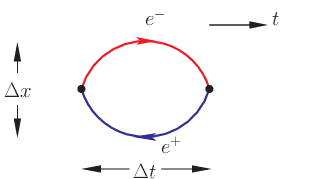
Fig. 1: Vacuum fluctuation into electron-positron pair.

Then, it is no surprise that if we exert a strong electric field $\vec E$ on the vacuum, the virtual electron and positron would be pulled in the opposite direction. As a net result, real electron and positron pairs can be created out of vacuum. Of course, the electric field has to be strong, to provide enough energy ($\gtrsim 2m_e c^2$) for the pair production. We can do an estimation as following. In order to create real particles, the electron and positron have to be pulled apart by at least one Compton length $\lambda_e = \frac{\hbar}{m_e c}$ (so that their wave packets do not overlap much). Over such a distance, the energy provided by the electric field is, $e E \lambda_e \ge 2 m_e c^2$. Therefore the threshold electric field is \[
E_\mathrm{th} \triangleq \frac{2 m_e c^3}{e\hbar} \simeq 10^{18} \, \mathrm{V/m}.
\]

Fig. 2: The Schwinger effect.

We can also look at the problem in another way (Fig. 2). In the Dirac theory, the vacuum is filled with negative energy electrons, known as the Dirac sea. In order to become physical, the electron has to get to the positive mass shell $E = \sqrt{\vec p^2 c^2 + m^2c^4}$. There is a $2 m_e c^2$ mass gap between them. (The Coulomb potential is negligible comparing to the mass gap.)

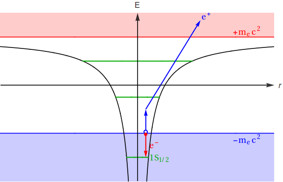
Fig. 3: The mass gap. The $x$-axis is the separation between the electron and its hole. Due to zitterbewegung, this distance can not be smaller than the Compton length.

Therefore, the creation of an electron (and the positron - the hole in the Dirac sea) can be viewed as a quantum tunneling process (Fig. 3). Then the external electric field turns the well to a barrier. The width of the barrier is proportional to $w \sim 2 m_e c^2/E$. According to WKB, the tunneling probability is \[
P \sim \exp\Big( - w \sqrt{2 m_e \times e (2m_e c^2) } \Big) \simeq \exp\Big( - E_\mathrm{th}/E \Big)
\]

Fig. 4: The electric field term the mass well to a barrier.

Super Critical Charge

We have seen in the last section that strong electric field can create electron-positron pairs out of vacuum. The Coulomb potential have a field strength proportional to $1/r^2$: $eE(r) = \frac{Z\alpha}{\hbar c r^2}$. Very close to the charge, the electric field would be extremely intense. So, it is natural to ask, if/why not such a phenomenon can be seen around a point charge. To achieve the threshold strength, the distance $r_\mathrm{th} = \sqrt{\frac{1}{2}Z\alpha} \lambda_e \simeq \sqrt{Z/2} \times 10^{-13}\,\mathrm{m}$ has to be large than the smallest distance between two particles.

For poin-like charged particles, such as electron, muons, the smallest distance is determined by 1). their Compton wavelength (zitterbewegung) $\lambda_\ell = \frac{m_e}{m_\ell}\lambda_e$; 2). the size of the bound state $\frac{m_\ell}{m\ell+m_e}\lambda_e/(Z\alpha)$. For electron/positron, this distance $r_\mathrm{th} = \sqrt{\alpha/2} \lambda_e$ is much smaller than their Compton wavelength. Therefore, even if such a phenomenon exists, it is included in the quantum fluctuation of the particle itself. Muon is about 207 times heavier than the electron. So its Compton wavelength is 207 times smaller than electron's. Then it is possible to produce a pair of real electron-positron. But as the pair were produced, the positron would be bound with the muon, forming a $\mu^-e^+$ atom.  However, the ground state radius of this atom $r \simeq a_0 = \lambda_e / \alpha \gg r_\mathrm{th}$. In other words, there is no enough energy to produce the electron-positron pair.  Similar cases happen for other leptons.

Fig. 5: The electron-positron pair production by a muon. This process is kinematically forbidden.

For composite systems, the charge factor $Z$ can be rather large. As a result, the possible bound state radius would decrease and the threshold radius increase (while the Compton wavelength remains the same). At some critical charge factor $Z_c \simeq 2/\alpha = 274$, the system would have enough energy to produce the electron-positron pair.

Again, Dirac Sea

To give a little bit quantitative touch, let's turn to the Dirac theory again (We don't turn to Schroedinger's theory because at the super critical charge, the system is relativistic.). The Dirac equation with a Coulomb potential produces the energy spectrum (Sommerfeld fine-structure formula): \[
E_{n,j} = mc^2 \left[ 1 + \frac{Z^2\alpha^2}{\left[n-j-\frac{1}{2} + \sqrt{(j+\frac{1}{2})^2-Z^2\alpha^2}\right]^2} \right]^{-1/2}
\] where $n = 1, 2, 3, \cdots$ is called the principal quantum number and $j=1/2, 3/2, 5/2, \cdots n-1/2$ is the total angular momentum. As we can see, for the S-state ($j=1/2$), the energy becomes imaginary if $Z > 1/\alpha \simeq 137$. This is half of the critical charge we found above using a crude estimate.

The existence of imaginary energy eigenvalues implies the Dirac Hamiltonian is no longer Hermitian as Dirac promised. Something is wrong. The solution of the Dirac equation does not represent the motion of an electron. Instead, given the time-dependent part $\exp\big(- |E|t \big)$, it represents the amplitude of some tunneling process.

Even though Dirac's theory is broken at $Z>137$, we can still mill some plausible physics out of it, invoking the Dirac sea -- as one may have noted, the creation of particles in the Dirac theory always involves the Dirac sea. It turns out, at the presence of the super critical charge, the Coulomb level dives into the Dirac sea. Therefore, the electrons at the Dirac sea jump down to Coulomb levels below and leave holes in the Dirac sea, manifested as the positron (see Fig. 6). This interpretation can be elaborated (including using other methods) to give the semi-quantitative dynamics of the process.

Fig. 6: The Dirac interpretation of the electron-positron pair production by a super critical charge.

QED with Strong External Fields

This problem can also be described by QED. Unlike the Dirac theory, the QED Hamiltonian is always Hermitian. Hence a self-consistent quantitative description of the problem has come from QED.

In QED, the vacuum is the ground state of the charge-zero sector:\[
H_\mathrm{QED} |\Omega\rangle = E_\Omega |\Omega\rangle
\] Here $H_\mathrm{QED}$ is the QED Hamiltonian. $E_\Omega$ is the vacuum energy. It can be renormalized to 0.

In our problem, there exists a charged heavy ion $Z^+$, which generates an strong electromagnetic field $\mathcal A$. With the presence of this field, the ground state may be different: \[
\big( H_\mathrm{QED} + J_\mu \mathcal A^\mu \big) |\Omega_{\mathcal A}\rangle = E_\mathcal{A} |\Omega_{\mathcal A}\rangle
\] Where $|\Omega_{\mathcal A}\rangle$ represents the polarized QED vacuum within field $\mathcal A^\mu$, $J^\mu = e\bar\psi \gamma^\mu \psi$ is the fermion charge current.

If the charge of the heavy ion is subcritical, the polarized vacuum only involves the photon loop-correction and electron loop-corrections (see Fig. 7), which can be taken into account by renormalization (UV renormalization and the bremsstrahlung) of the heavy ion. When the mass of the heavy ion is sufficiently large, the renormalization effects can be neglected. When the charge of the heavy ion $Z^+$ exceeds some critical value $Z_c$, a new vacuum state emerges. It consists a free positron and a $Z^+e^-$ bound-state. Such a vacuum state is called a charged vacuum. Dynamically, we see the spontaneous production of an electron-positron pair.

Fig. 7: The QED vacuum within the subcritical (top) and supercritical (bottom) external field. The double line represent the heavy ion with a positive subcritical charge. The single line loop represents the electron/positron loop correction. The wavy lines represents the photons. The dot represents the coupling between the photon and the super critical charge. The blue single line represents the emitted positron. The red single line represents the bound electron.

In practice, the matrix can be truncated to the first few sector to retain the minimal physical of the charged vacuum (See Fig. 9). The minimal sector should include at least one photon and one pair of electron and positron.

Fig. 9: The QED matrix within the first few Fock sectors. The vertex with a dot represents the super critical charge coupling $Ze$.

We can further suppress the heavy ion sector and treat the field it generates simply as a classical external field. In this way the charged vacuum is more qualified for its name. (Otherwise it is just the ground state of the supercritical charge sector.)

Fig. 10: (left panel) the vacuum polarization within a subcritical potential; (right panel) the pair production (the charged vacuum) within a supercritical potential.

The charged vacuum can also be studied within the path integral formalism. According to this formalism, the vacuum expectation value of an operator within the external field is, simply, \[
\langle \mathrm T\mathcal O_\psi \rangle_{\mathcal A} = \int \mathcal D_{\psi,\bar\psi, \mathcal A} \, \mathcal O_\psi \, \exp\Big[ i\int d^4x \, \bar \psi(x) \big( i\gamma^\mu D_\mu - m\big) \psi(x)\Big]
\] where $D_\mu = \partial_\mu - ie\mathcal A_\mu$.

Both the matrix diagonalization and the path integral methods are non-perturbative. But different approximation may arise for each formalism. We shall not delve into those lengthy technologies but only mention one famous result due to Schwinger. Let's consider the production rate, which is related to the vacuum decay probability: $P = 1 - |\langle\Omega_{\mathcal A}|\Omega_{\mathcal A}\rangle|^2 \approx 1 - \exp( -2 \mathrm{Im} S_\mathrm{eff})$. Here Schwinger applied an approximation: $\langle\Omega_{\mathcal A}|\Omega_{\mathcal A}\rangle = \det^{-1} \bar\psi \big( i\gamma^\mu D_\mu - m\big) \psi \approx \exp(i S_\mathrm{eff})$. $S_\mathrm{eff}=\int d^4x\,\mathcal L_\mathrm{eff}$ is called the effective action. The one-loop effective action was calculated obtained Heisenberg and Bonn. Plug into this effective action, and assuming a uniform electric field $E$, Schwinger's conclusion for the vacuum pair production rate is, \[
R \triangleq \frac{dN}{dVdt} = \frac{(eE)^2}{4\pi^3}\sum_{n=1}^\infty \frac{1}{n^2} \exp\big( -n\pi E_c/E\big)
\] where $E_c \triangleq m_e^2 c^3/(e\hbar) \sim 10^{18} \,\mathrm{V/m}$ is the critical electric field. This formulation is the famous Schwinger mechanism of vacuum pair production.


One can also solve the Schroedinger's equation directly, starting for example, from the normal QED vacuum state: \[
 i \frac{\partial}{\partial t} |\psi(t)\rangle = \big( H_\mathrm{QED} + J^\mu \mathcal A_\mu\big) | \psi(t)\rangle, \quad
 |\psi(0)\rangle = |\Omega\rangle.
\] In this way, the time evolution of the QED vacuum can be studied. This approach is also non-perturbative.

In the above description, we deliberately avoid the photon mediated electron-positron interaction. This can be included by the quantized electromagnetic field $A^\mu$. So the full covariant derivative can be written as $D_\mu = \partial_\mu - i e\mathcal A_\mu - ie A_\mu$. Note that this field is small comparing with the external field $\mathcal A$ generated by the supercritical heavy ion, $|\mathcal A| \sim Z |A|$. In practice, the correction due to quantized photon can be included through the usual perturbation theory.

Fig. 11: the same diagrams as Fig. 10, but taking into account the quantized photons. The external fields are represented as double wavy lines. The real photon lines are the single wavy lines.

Pair Production in the Relativistic Heavy Ion Collisions

Experiments

[ To Be Continued ... ]

---

References:

[1]: W. Greiner, B. Muller and J. Rafelski, Quantum electrodynamics of strong fields, (1985) Springer-Verlag, Berlin Heidelberg.

Disturbing a Quantum Field

Lesson from Condensed Matter Physics (CMP)

In condensed matter systems, it is useful to study the collective response to external fields. For example, when adding an electric field $\vec E$ to a metal, a current $\vec J$ would be generated. We call the response the conductivity, which is unique for each material, thus reflects internal properties of the system. Quantitatively, the conductivity is defined in terms of the external field and the respond current \[
J(t, \vec x) = \int \mathrm d^3x' \int_{-\infty}^t \mathrm dt' \sigma(t-t', \vec x - \vec x') E(t', \vec x').
\] The upper limit of the temporal integral is due to causality. In general, the conductivity may depends on the external field $\vec E$ (non-linear effect). In the weak field limit $E \to 0$,  however, it is independent to $E$ (linear response) and provides an important probe for the property of the material. There are also other linear responses of the condensed matter systems. The Green-Kubo formula (Melville Green 1954, Ryogo Kubo 1957) provides a neat recipe to compute the linear response of the condensed matter system to an external field.

Suppose a weak external field $F(t, \vec x)$ couples to a condensed matter system through $H_\mathrm{int} = \int \mathrm d^3x F(t, \vec x) A(t, \vec x)$. The system was originally described by the density operator $\varrho =Z^{-1} \exp \big[ -\beta (H - \mu N) \big]$, where $Z = \mathrm{tr} \exp \big[ -\beta (H - \mu N) \big]$. The linear response theory concerns the expectation value of an observable $B(t, \vec x)$: \[
\langle  B(t, \vec x) \rangle_F - \langle  B(t, \vec x) \rangle= \mathrm{tr} \left[ \big(\varrho_F(t)-\varrho(t)\big) B(t, \vec x) \right] \equiv \int \mathrm dt' \int \mathrm d^3x' \chi_{AB}(t-t',\vec x-\vec x') F(t', \vec x')
\] where $\varrho_F(t)$ is the density matrix in the perturbed system. The Green-Kubo formula asserts that the linear transportation coefficient \[
\chi_{AB}(t-t', \vec x - \vec x') = -i \Theta(t-t') \langle [B(t, \vec x), A(t', \vec x')] \rangle.
\] For example, the conductivity is related to the current-current correlation function*, \[
\sigma_{AB}(t-t', \vec x - \vec x') = -i \Theta(t-t') \langle [\partial_t^{-1}J(t, \vec x), \partial_{t'}^{-1}J(t', \vec x')] \rangle.
\]

*In general, the current is a four-vector hence the response is a tensor. One should consider the contribution from all components, which gives rise to several transport coefficients: the longitudinal conductivity, the density responses as well as the Hall conductivity etc.

Quantum Field Theory (QFT)

The vacuum state of QFT $|\Omega\rangle$ is intrinsically many-body (even the free field theory!). Let's disturb the QFT vacuum and measure the linear response.

Let $J_r(x)$ be a classical source. We couple it to the quantum field $\varphi(x)$ through $\mathscr H_\mathrm{int}(x) = A_r(x) J_r(x)$, where $A$ is a local operator constructed from $\varphi$. Then we measure the vacuum expectation value (VEV) of an observable $B_s(x)$ (To measure this observable, we may, for example, couple the field to a classical field. That's why we often consider the case $A = B$, which we sill talk about later.): $\langle B_s(x) \rangle_J \equiv Z_J^{-1} \langle \Omega | B_s(x) | \Omega \rangle_J$, where $Z_J = \langle \Omega | \Omega\rangle_J$ is the perturbed partition function. In the weak source limit ($J\to 0$), the response should be linear, similar to the condensed matter system: \[
\langle B_s(x) \rangle = \int \mathrm d^4 x' \chi_{sr}^{BA}(x,x') J_r(x') + \mathcal O(J^2).
\] Let $Z$ be the unperturbed partition function. In the weak external field limit $J \to 0$, \[
Z_J = Z \Big(1 - i \int \mathrm d^4x \langle A_r(x) \Omega \rangle J_r(x) - \frac{1}{2} \int \mathrm d^4x\mathrm d^4y \langle \mathcal T\big\{ A_r(x) A_s(y) \big\} \rangle J_r(x) J_s(y) \Big).
\] and $\langle \Omega | B_s(x) | \Omega \rangle_J$ is, \[
 \langle \Omega | B_s(x) | \Omega \rangle_J = \langle \Omega | B_s(x) | \Omega \rangle
  -i \int \mathrm d^4 x' \langle \Omega | \mathcal T \big\{B_s(x)A_r(x')\big\} | \Omega\rangle J_r(x').
\] Then the vacuum expectation value (VEV) \[
\langle B_s(x) \rangle_J
= \langle B_s(x) \rangle + i \int \mathrm d^4x' \langle A_r(x') \rangle \langle B_s(x) \rangle J_r(x') - i \int \mathrm d^4 x' \langle \mathcal T \big\{B_s(x) A_r(x')\big\} \rangle J_r(x').
\] It is convenient to work with "renormalized" operators that have vanishing VEV without the presence of the external source. For example, we may define: $B^R_s(x) = B_s(x) - \langle B_s(x)\rangle$. It is easy to see,\[
\langle B^R_s(x) \rangle_J
=- i \int \mathrm d^4 x' \langle \mathcal T \big\{B^R_s(x) A^R_r(x')\big\} \rangle J_r(x').
\] Therefore, the transport coefficient $\chi(x,x') \propto \langle \mathcal T \big\{B^R_s(x) A^R_r(x')\big\} \rangle$. Note that causality is preserved by time-ordering operator $\mathcal T$.

From now on, we'll assume all the operators have been properly renormalized, unless elsewhere stated.

Example 1: Field Propagation

$A = B = \varphi$, where $\varphi(x)$ is the renormalized field such that $\langle \Omega |\varphi(x)|\Omega\rangle = 0$. $\langle\varphi(x)\rangle_J$ represents the amplitude for finding a physical particle in the disturbed vacuum. \[
\langle\varphi_a(x)\rangle_J =- i \int \mathrm d^4 x' \langle \mathcal T \big\{\varphi_a(x) \varphi_b(x')\big\} \rangle J_b(x'),
\] Here $D_{ab}(x-x') \equiv i\langle \mathcal T \big\{\varphi_a(x) \varphi_b(x')\big\} \rangle$ is nothing but the Feynman propagator. This means sense physically: the classical source $J$ creates a physical particle at $x'$, and then the particle propagate to $x$ to be detected.

Note that we are not doing perturbation theory. The graphical representations are not necessarily Feynman diagrams.

Example 2: Vacuum Polarization

Let $A = B = J^\mu(x)$, where $J^\mu$ is the electromagnetic current. We couple a classical electromagnetic field $\mathcal A_\mu(x) e^{-\epsilon |x^0|}, (\epsilon\to 0^+)$ to the vacuum and measure the current: \[
\langle J^\mu(x) \rangle_{\mathcal A} = -i \int \mathrm d^4x' \left< \mathcal T \big\{J^\mu(x)J^\nu(x') \big\}  \right> \mathcal A_\nu(x') e^{-\epsilon |x'^0|}.
\] The linear transport coefficient is called the polarization tensor: \[
\Pi^{\mu\nu}(x-x') \equiv \left< \mathcal T \big\{J^\mu(x)J^\nu(x') \big\}  \right>.
\] Consider a free Dirac field, \[
\psi(x) = \sum_{s=\pm} \int\frac{\mathrm d^3 k}{(2\pi)^32\omega_p} \Big[ u_s(k) b_s(k) e^{ik\cdot x} + v_s(k) d^\dagger_s(k) e^{-ik\cdot x} \Big].
\] The electromagnetic current is $J^\mu(x) = \bar\psi(x)\gamma^\mu\psi(x)$. Applying Wick theorem, the polarization tensor is \[
\Pi^{\mu\nu}(x-x') = \mathrm{tr} \Big[ \gamma^\mu S(x-x') \gamma^\nu S(x-x')  \Big] - \mathrm{tr} \Big[\gamma^\mu S(x-x)\Big] \mathrm{tr} \Big[\gamma^\nu S(x'-x')\Big].
\]

Now consider a perturbative spinor electrodynamics. Let's denote the free Dirac action as $S_0$, the
interaction as $S_\mathrm{int} = \int\mathrm d^4x \bar\psi(x)\gamma^\mu\psi(x) A_\mu(x)$.

 

Here we are only concerning the linear effect. One may well ask the question of the induced current by a strong classical source field. The problem is called the Schwinger effect. It turns out, in the semi-classical approximation, the partition function is \[
Z_\mathcal{A} \equiv \langle \Omega | \Omega \rangle_\mathcal{A}  \approx e^{iS_\mathrm{eff}} \] Therefore, the pair production probability (or rather the vacuum decay probability) \[
P = 1 - e^{-2\mathrm{Im}S_\mathrm{eff}}. \] Considering only the one-loop effect in a constant E-field, Schwinger calculated the vacuum decay rate (Phys. Rev. 82, 664 (1951)), \[
\frac{\mathrm dN}{\mathrm dV \mathrm dt} = \frac{(eE)^2}{4\pi^3}\sum_{n=1}^\infty \frac{1}{n^2} e^{-n\pi E_c/E} \] where $E_c = \frac{m_e^2c^3}{e\hbar} \sim 10^{18} \text{V/m}$ is a super-duperly strong field! However, it may be found in: a) heavy ion collision; b) magnetar; c) condensed matter emulated QED (e.g., graphene); d) high energy lasers (still a long way to go).

Example 3: Hadron Structure

Let $A = B = J^\mu(x)$, where $J^\mu$ is the electromagnetic current. The linear response can also be used to study a bound state. The key is to "create" and "annihilate" a bound state from the vacuum with the field operator, \[
|\psi(z)\rangle \equiv \lim_{z^0\to-\infty}\psi(z) |\Omega\rangle, \\
\langle\psi(y) | \equiv \lim_{y^0\to+\infty} \langle \Omega | \bar\psi(y).
\] We couple a classical electromagnetic field $\mathcal A_\mu(x) e^{-\epsilon |x^0|}, (\epsilon\to 0^+)$ to a physical particle through the minimal coupling $\mathcal A_\mu J^\mu$. Then we measure the charge distribution: \[
\langle \psi(y) | J^\mu(x) |\psi(z)\rangle_{\mathcal A} = -i \int \mathrm d^4x' \left< \psi(y)\right| \mathcal T \big\{J^\mu(x)J^\nu(x') \big\} \left| \psi(z)\right> \mathcal A_\nu(x') e^{-\epsilon |x'^0|}
\] The particle propagation before and after the experiment is no interest to us. Let's do Fourier transform:\[
\psi(z) |\Omega\rangle = \int \frac{\mathrm d^3 p}{(2\pi)^32\omega_p} \tilde\psi(p) e^{ip\cdot x} |p,\sigma\rangle, \quad (\omega_p = \sqrt{m^2+\mathbf p^2})
\] Therefore, let's study the current distribution of plane wave modes: \[
\langle p',\sigma' | J^\mu(x) | p,\sigma \rangle_{\mathcal A} = -i \int \mathrm d^4x' \langle p',\sigma' | \mathcal T \big\{J^\mu(x)J^\nu(x') \big\} | p,\sigma \rangle \mathcal A_\nu(x') e^{-\epsilon |x'^0|}
\]

Beyond Linear Response

The linear response can be use to formulate the perturbation theory. Let's disturb a scalar field $\varphi(x)$ with a classical source $j$. The new partition function is, \[
\begin{split}
Z_j &= \int \mathcal D_\varphi \, \exp \Big( iS + i\int\mathrm d^4x\, j(x) \varphi(x) \Big)
=\langle\Omega\mid \mathcal T \exp\Big( i\int \mathrm d^4x\, j(x)\varphi(x)\Big) \mid \Omega\rangle\\
&= \sum_{n=0}^\infty \frac{i^n}{n!}\int\mathrm d^4x_1\,\cdots\mathrm d^4x_n\, j(x_1) \cdots j(x_n) \langle\Omega\mid\mathcal T\varphi(x_1)\varphi(x_2)\cdots \varphi(x_n)\mid\Omega\rangle \\
&= \sum_{n=0}^\infty \frac{i^n}{n!}\int\mathrm d^4x_1\,\cdots\mathrm d^4x_n\, j(x_1) \cdots j(x_n) G(x_1, x_2, \cdots, x_n)
\end{split}
\] where $G(x_1,x_2,\cdots,x_n) = \langle\Omega\mid\mathcal T\varphi(x_1)\varphi(x_2)\cdots \varphi(x_n)\mid\Omega\rangle$ is the $n$-point correlation function (aka. $n$-point causal correlator). The translational symmetry implies $G(x_1,\cdots,x_n) = G(x_1-a,\cdots,x_n-a)$. In the momentum space, \[
G(x_1, \cdots, x_n) = \int\frac{\mathrm d^4p_1}{(2\pi)^4} \cdots \frac{\mathrm d^4p_n}{(2\pi)^4} \exp\Big( ip_1\cdot x_1+\cdots + ip_n\cdot x_n\Big) G(p_1,\cdots,p_n)
\] The translational symmetry implies $G(p_1,\cdots,p_n) = (2\pi)^4\delta^4(p_1+\cdots+p_n)\tilde G(p_1,\cdots,p_n)$.

The correlators $G(x_1,x_2,\cdots,x_n)$ can be represented by the sum of graphs subject to $n$ external legs, $G(x_1,\cdots,x_n) = \sum_{g} D_g(x_1,\cdots, x_n)$, known as the Feynman diagrams.

A diagrammatic representation of a n-point causal correlator

Next, it is convenient to work with the irreducible diagrams (represented by connected graphs), $C$, and the corresponding correlator $G_c(x_1,x_2,\cdots,x_n)$. Apparently, any diagram $D_g$ with topology $g$ can be written as a product of its connected components, \[
\frac{1}{n_g!} \frac{i^{n_g}}{|\mathrm{Aut}\,g|}\int\mathrm d^4x_1\,\cdots\mathrm d^4x_{n_g}\, j(x_1) \cdots j(x_{n_g}) D_g(x_1, \cdots, x_{n_g}) \\
=  \prod_{s\in S_g} \frac{1}{m_s!} \bigg( \frac{1}{n_s!}\frac{i^{n_s}}{|\mathrm{Aut}\, s|}\int\mathrm d^4x_1\,\cdots\mathrm d^4x_{n_g}\, j(x_1) \cdots j(x_{n_g}) D_s \bigg)^{m_s}
\] where $S_g$ be the set of connected subgraphs of graph $g$, $m_s$ is the multiplicity of $s\in S_g$ in $g$, that is, $g$ consists of $m_s$ copies of $s$; $n_s$ evaluates the number of external legs in graph $s$ and $n_g = \sum_{s\in S_g} m_s n_s$. The factor $\frac{1}{n_s!}$ came from the multinomial coefficients ${n_g \choose n_{s_1}, n_{s_2}, \cdots}}$, which represents the number of ways to split the $n_g$ external sources.

Then the disturbed partition function $Z_j$, \[
\begin{split}
Z_j &= \sum_{n=0}^\infty \frac{i^n}{n!}\int\mathrm d^4x_1\,\cdots\mathrm d^4x_n\, j(x_1) \cdots j(x_n) G(x_1, \cdots, x_n) \\
&= \sum_{n=0}^\infty \frac{i^n}{n!} \int\mathrm d^4x_1\,\cdots\mathrm d^4x_n\, j(x_1) \cdots j(x_n) \sum_{g, n_g=n} \frac{1}{|\mathrm {Aut}\,g| } D_g(x_1, \cdots, x_n) \\
&= \sum_{g} \prod_{s\in S_g} \frac{1}{m_s!} \bigg(\frac{1}{n_s!}\frac{i^{n_s}}{|\mathrm{Aut}\, s|} \int\mathrm d^4x_1\,\cdots\mathrm d^4x_{n_s}\, j(x_1) \cdots j(x_{n_s}) D_s \bigg)^{m_s} \\
\end{split}
\] In the last line, $s \sim \frac{1}{n_s!}\frac{i^{n_s}}{|\mathrm{Aut}\, s|} \int\mathrm d^4x_1\,\cdots\mathrm d^4x_{n_s}\, j(x_1) \cdots j(x_{n_s}) D_s$ is the expression for connect graph $s$. Compare the last line with multinomial expansion $(x_1+x_2+\cdots + x_k)^n = \sum_{m_1,m_2,\cdots,m_k} {n \choose m_1,m_2,\cdots,m_k} x_1^{m_1}x_2^{m_2}\cdots x_k^{m_k}$. Therefore, we can change the order of summation and multiplication and \[
Z_j = \exp \sum_{n=0}^\infty \frac{i^n}{n!} \int \mathrm d^4x_1\,\cdots\mathrm d^4x_n\, j(x_1) \cdots j(x_n) \sum_{g\in C, n_c=n} D_c(x_1,x_2,\cdots,x_n).
\] Here $C$ is the collection of all connected Feynman diagrams. This result is the linked cluster theorem, which relates the free energy with the connect diagrams, \[
iW_j = \ln Z_j = \sum_{n=0}^\infty \frac{i^n}{n!}\int\mathrm d^4x_1\,\cdots\mathrm d^4x_n\, j(x_1) \cdots j(x_n) G_c(x_1, x_2, \cdots, x_n).
\] This theorem can be proven more rigorously from induction, by defining the connected correlator $G_c(x_1, \cdots, x_n) = G(x_1, \cdots, x_n) - \sum_{P}\prod_{p\in P} G_c(\{x\}_p)$.

Consider the vacuum expectation value (VEV) of the field $\varphi(x)$, \[
\langle \varphi(x) \rangle_j = Z_j^{-1} \frac{1}{i}\frac{\delta}{\delta j(x)} Z_j
= \frac{\delta}{\delta j(x)} W_j
\] Let's do a Legendre transformation to introduce a new quantity (the minus sign is the convention): \[
-\Gamma_j = \int \mathrm d^4x\, \delta/\delta j(x) W_j \cdot j(x) - W_j
\]

$\beta$ and $\gamma^0$

$\gamma^0$ with the other three gamma matices $\vec\gamma$, furnishes a representation of the Clifford algebra $\mathrm{C\ell}_{1,3}(\mathbb R)$ \[\{ \gamma^\mu, \gamma^\nu \} = 2 g^{\mu\nu}, \] where $\{X, Y\} = XY + YX$, $g^{\mu\nu}$ is the Minkowski space metric.

The parity matrix $\beta$ is a spinor representation of the parity operator: \[
P^{-1} \Psi(x) P = \beta \Psi(\mathcal P\cdot x)
\] where $\mathcal P^\mu_\nu = \mathrm{diag}\{1, -1, -1, -1\}$ is the 4-vector representation of the parity operator. The operator $P$ here, of course, furnishes a field representation, with the help of $\beta$ and $\mathcal P$. Then $\beta$ satisfies the parity relations: $\beta^2 = 1$, $\beta^{-1} \vec\gamma \beta = -\vec\gamma$, $\beta^{-1} \gamma^0 \beta = \gamma^0$.

It is popular to take $\beta = \gamma^0$. But this may not always be the correct one. The reason is the metric tensor g. There are two popular sign conventions of $g^{\mu\nu}$: $\mathrm{diag}\{+1, -1, -1, -1\}$ and $\mathrm{diag}\{-1, +1, +1, +1\}$. Under the first convention, $\gamma^0 \gamma^0 = 1$. $\beta$ is readily to be chosen as $\gamma^0$. It is easy to check all the parity relations are satisfied. Under the second conventions, however, $\gamma^0 \gamma^0 =-1$, which means $\beta$ should be $\pm i\gamma^0$.

Of course, all unitary representations in quantum theory is only determined up to an over all phase factor: \[
P^{-1} \Psi(x) P = \exp(i\eta) \beta \Psi(\mathcal P\cdot x), \quad (\eta \in \mathbb R)
\] It is possible to choose phase factors such that $\beta = \gamma^0$ always holds. For example, for $g_{00} = +1$, we choose $\exp(i\eta) = 1$; for $g_{00}=-1$, we choose $\exp(i\eta) = i$. This is essentially what is done in the literature, such as Peskin & Schroeder, Mark Srednicki etc. But keep in mind that, the phase factors for T, C, and P are not all independent. It is important to be self-consistent at the end of the day. Weinberg's book keeps the phase factors open.

Charge Symmetry

Classical Example

Under the charge conjugation (C for short), charge $q \to -q$, electric field $\mathbf E \to - \mathbf E$, but the solution of the dynamical equation, the position vector, remains invariant $\mathbf r(t) \to \mathbf r(t)$.

In the theories particle and antiparticle do not mix (e.g. Schroedinger's Equation, Pauli's Equation), charge symmetry is almost trivial.

Dirac Theory

Dirac equation, \[
(i\partial_\mu \gamma^\mu - eA_\mu\gamma^\mu + m)\psi(x) = 0
\] describes the relativistic motion of electrons as well as positrons. $e = 1.602176565(35)\times 10^{-19} \mathrm{C}$ is just a positive number, so-called elementary charge. In general, the solution $\psi(x)$ contains both the electron state and the positron state. Here we take $g_{\mu\nu} = \mathrm{diag}\{-,+,+,+\}$.

In free particle theory where $A = 0$, there are four independent plane wave solutions: two positive energy solutions describe electrons $u_s(p) e^{+ip\cdot x}, \; s=\pm\frac{1}{2}$ and two negative energy solutions describe the positrons $v_s(p) e^{-ip\cdot x},\; s=\pm\frac{1}{2}$, $E_{\mathbf p} = \sqrt{\mathbf p^2+m^2}$. A general solution (a wave packet) is a superposition of the two pieces: $\psi(x) \equiv \psi^+(x) + \psi^-(x)$ where \[
\psi^+(x) = \sum_{s=\pm}\int \frac{\mathrm{d}^3p}{(2\pi)^32E_{\mathbf p}} b_s(\mathbf p) u_s(p) e^{+ip\cdot x}, \\
\psi^-(x) = \sum_{s=\pm}\int \frac{\mathrm{d}^3p}{(2\pi)^32E_{\mathbf p}} d^*_s(\mathbf p) v_s(p) e^{-ip\cdot x}. \] $b, d^*$ are some c-number smooth functions.

As a relativistic wave function approach, the charge conjugation would be implemented as a "unitary" spinor matrix: $C \bar C \triangleq C (\beta C^\dagger \beta) \equiv 1$. This matrix should transform a plane wave electron to a plane wave positron or vice versa, i.e. $C u_s(p)e^{+ip\cdot x} \sim v_s(p) e^{-ip\cdot x}$. We can immediately see that this is not possible if the charge conjugation spares the exponential function. We conclude that in Dirac theory, the charge conjugation must be implemented as an anti-unitary spinor operator. Thus, we require \[
C \left( u_s(p) e^{+ip\cdot x}\right) =\eta_c v^*_s(p) e^{-ip\cdot x} \\
C \left( v_s(p) e^{-ip\cdot x} \right) = \xi_c u^*_s(p) e^{+ip\cdot x} \] where $|\eta_c| = |\xi_c| = 1$. For simplicity, we'll take these constant phases to unity. The charge conjugated field is denoted as, \[
C\psi(x) \equiv \psi^c(x) = \sum_{s=\pm}\int \frac{\mathrm{d}^3p}{(2\pi)^32E_{\mathbf p}} \Big[ b^*_s(\mathbf p) v^*_s(p) e^{-ip\cdot x} + d_s(\mathbf p) u^*_s(p) e^{+ip\cdot x} \Big]
\]
It is conventional to define the unitary part of $C$ by a new spinor matrix $\mathcal C$ (curly C),
\[ C \psi(x) \triangleq \mathcal C \beta \psi^*(x) \equiv \mathcal C \bar\psi^T(x) \] (Here adding a $\beta$ is just a convention.). It is easy to see, $\mathcal C$ is unitary $\mathcal{C} \bar{\mathcal{C}}= 1$. An example of the choice of $\mathcal C$ is (Srednicki p. 242, 2007), \[
\mathcal C =
\begin{pmatrix}
0 & -1 & 0 & 0 \\
+1 & 0 & 0 & 0 \\
0 & 0 & 0 & +1 \\
0 & 0 & -1 & 0
\end{pmatrix}
\] The theory must be invariant under the charge conjugation, or $\mathcal L \overset{C}{\to} \mathcal L$, which implies $\mathcal C \gamma_\mu = - \gamma_\mu^T \mathcal C$. Applying to the $u,v$ spinors, $\mathcal C \bar u^T_s(p) = v_s(p), \mathcal C \bar v^T_s(p) = u_s(p)$.

Heuristically, the transformation can be viewed as a two-step procedure:

1. swap the particle species, by exchanging $u_s(p)$ and $v_s(p)$ (and of course also the sign of the charge);
2. reverse the time, by conjugating the exponential factor. 

As stated before, the E&M field transforms under the charge conjugation as $A^\mu \overset{C}{\to} -A^\mu$. Then the charge conjugated of the Dirac wave equation is: \[
(i\partial_\mu \gamma^\mu {\color \red +} eA_\mu\gamma^\mu + m){\color \red {\psi^c(x)}} = 0
\] Note the sign change. It is easy to check that if $\psi(x)$ satisfies the original Dirac wave equation,
$\psi^c(x)$ satisfies this equation, which just confirms that the Dirac theory is invariant under the charge conjugation.

To compare with the classical charge conjugation, the dynamical equation (the equation of motion) is still invariant under the charge conjugation. But the solution of it would change under the charge conjugation, $\psi(x) \overset{C}{\to} \psi^c(x)$.

Quantum field theory

In quantum field theory, charge conjugation is implemented as a unitary operator, which we shall call $C$ (not be confused with the anti-unitary spinor operator introduced in the previous section). The definition is simple (We have also taken a particular choice of a possible phase factor. See Weinberg, 2005): \[
C^{-1} b_s(p) C = d_s(p), \quad C^{-1} d_s(p) C = b_s(p), \quad C^{-1} a_\lambda(p) C = - a_\lambda(p), \] where $b_s(p), d_s(p), a_\lambda(p)$ are the electron, positron and photon annihilation operators, respectively.

For the free Dirac field, \[

\psi(x) = \sum_{s=\pm}\int \frac{\mathrm{d}^3p}{(2\pi)^32E_{\mathbf p}} \Big[ b_s(\mathbf p) u_s(p) e^{+ip\cdot x} + d^\dagger_s(\mathbf p) v_s(p) e^{-ip\cdot x} \Big].
\] It can be shown, after some algebra (e.g., Srenicki p.225) that for the quantum fields, \[

C^{-1} \psi(x) C = \mathcal C \bar\psi^T(x) \equiv  \psi^c(x), \quad C^{-1} A^\mu(x) C = - A^\mu(x), \quad C^{-1}\varphi(x)C = \varphi^*(x). \] Then, it can be shown immediately that the Lagrangian is invariant under the charge conjugation.

Alot of notations are abused, although they are different quantities (quantum field theoretical vs. Dirac relativistic wavefunctional). Superficially, this resembles the Dirac equation result introduced in the previous section, although we should point out that here $\psi(x)$ is a field operator instead of a relativistic wave function. But this similarity means that we can do it one way or another. The same answer would be obtained. That's also the reason of the heavy abuse of notations.


To compare with the classical case and the Dirac case, the solution of the dynamical equation changes, $\psi(x) \overset{C}{\to} \psi^c(x)$. Notation-wise, this is similar to the Dirac case. See Table 1.

Table 1

Figure 1. $\langle p s \left| J^\mu(x) \right| p' s'\rangle \equiv e^{-i(p-p')\cdot x} \bar u_s(p)e \Gamma^\mu u_{s'}(p')$

A theory invariant under charge conjugation does not automatically implies a symmetric solution. The symmetry could be broken by either explicit theory (e.g. weak interaction, $\theta$-term etc.), or spontaneous symmetry breaking. In general, the charge distribution, the matrix element of the charge current operator between two physical states can be written as, \[
\langle p s \left| J^\mu(x) \right| p' s' \rangle \equiv e \bar u_s(p) \Gamma^\mu u_{s'}(p') \exp[-i(p-p')\cdot x].
\] Here $\Gamma^\mu = \Gamma^\mu(p-p')$ is some spinor operator. $\Gamma^\mu$ can be represented by the spinor basis, \[ \Gamma^\mu(q) = F_1(q^2) \gamma^\mu + F_2(q^2) \frac{i}{2m_e} \sigma^{\mu\nu} q_\nu + F_3(q^2) \frac{1}{2m_e}\gamma_5 \sigma^{\mu\nu} q_\nu,
\] here $q = p-p'$, $\sigma^{\mu\nu} = \frac{i}{2} [ \gamma^\mu, \gamma^\nu ]$. Under the charge conjugation,
$\gamma^\mu \overset{C}{\to} \mathcal C^{-1}(\gamma^\mu)^T \mathcal C = -\gamma^\mu$;
$\sigma^{\mu\nu} \overset{C}{\to} \mathcal C^{-1}(\sigma{^\mu\nu})^T \mathcal C = -\sigma^{\mu\nu}$;
$\gamma_5\sigma^{\mu\nu} \overset{C}{\to}\mathcal C^{-1}(\gamma_5\sigma{^\mu\nu})^T \mathcal C = -\gamma_5\sigma^{\mu\nu}$.

The first term corresponds to charge with the charge normalization $F_1(0) = 1$. The second term represents the magnetic moment. $F_2(0) = \frac{\alpha}{2\pi} + \mathcal O(\alpha^2)$. The third term represents an electric dipole moment $d_e = \left|\frac{1}{2m_e}F_3(0)\right| < 10^{-27} e\cdot$ cm.

On the Spin in Relativistic Dynamics

Spin is an intrinsic property of a particle associated with rotational symmetry. Roughly speaking, it is the intrinsic part of the angular momentum. Measurement of angular momentum $\vec{J}$ differs in different reference frames. It is tempted to decompose it $\vec{J} = \vec{L} + \vec{S}$, where $\vec{L}$ called orbital angular momentum, $\vec{S}$ called spin angular momentum or spin for short. Orbital angular momentum should vanish in the particle rest frame $\vec{P} = 0$. In non-relativistic quantum mechanics, it is defined as $\vec{L} = \vec{X} \times \vec{P}$. But it is not clear a priori that such a decomposition is always available in relativistic dynamics. Another way of defining spin, is to measure the angular momentum in the particle rest frame. In relativistic dynamics, there is no unique Lorentz transformation that transforms a momentum state to the particle rest frame. Ambiguity thus exists for the definition of spin.

Nevertheless, spin can be defined formally as a vector operator that satisfying the following conditions: \[ \left[ S^i, S^j \right] = i\varepsilon^{ijk} S^k; \quad (i,j,k = 1,2,3) \\ \left[ S^i, P^j \right] = 0; \qquad \qquad \qquad \qquad \quad (\mathbf{*})\\ \vec{S} = \vec{J} \qquad \text{ if } \vec{P} = \vec{p}_c. \qquad \qquad \] The last condition should be understood within momentum states $\vec{S} \left.| p, \sigma\right> = \vec{J} \left.| p, \sigma\right> \quad \text{if } \vec{p} = \vec{p}_c$. The spin operator $\vec{S}$ described above is not covariant. The canonical example of $\vec{p}_c$ is $\vec{0}$.

Spin as an operator must also depend on the specific realization of the space-time symmetry (the Poincaré symmetry), i.e. the representation. According to Wigner theorem, a symmetry transformation in quantum mechanics should be realized either as unitary operator or as anti-unitary operator. Because Lorentz group is non-compact, all unitary representation has to be infinite dimensional, namely fields. Nevertheless, a relativistic theory still can have a finite-dimensional representation. The prominent example is the Dirac theory of relativistic electrons.

Poincaré algebra

Consider the Poincaré algebra, \[
\left[ P^\mu, P^\nu \right] = 0; \qquad \qquad \qquad \qquad \qquad \qquad \qquad \qquad \\
\left[ P^\lambda, M^{\mu\nu} \right] = i \left( g^{\lambda\mu} P^\nu - g^{\lambda\nu} P^\mu \right); \quad \qquad \qquad \qquad \qquad \quad \\
\left[ M^{\lambda\rho}, M^{\mu\nu} \right] = i\left( g^{\lambda\nu} M^{\rho\mu} + g^{\rho\mu} M^{\lambda\nu} - g^{\lambda\mu}M^{\rho\nu} - g^{\rho\nu} M^{\lambda\mu} \right);
\] $P^\mu$ and $M^{\mu\nu}$ are the 10 generators of the Poincaré algebra. The six independent components of $M^{\mu\nu}$ are, $J^k \equiv \frac{1}{2} \epsilon^{ijk}M^{ij}, (i,j,k = 1,2,3)$ the angular momenta; $K^i \equiv M^{0i}, (i = 1,2,3)$ the boosts.

The metric tensor is \[
g^{\mu\nu} = g_{\mu\nu} = \begin{pmatrix} 1 & & & \\ & -1 & & \\ & & -1 & \\ & & & -1 \\ \end{pmatrix}
\]
$P^2 = P_\mu P^\mu = \mathscr{M}^2$ is a Casimir element, known as invariant mass squared. In this post, we only consider massive case $\mathscr{M}^2 > 0$ for simplicity.

Pauli-Lubanski Pseudo Vector

\[ W^\mu = -\frac{1}{2} \varepsilon^{\mu\nu\kappa\rho} M_{\nu\kappa} P_\rho, \] where $\varepsilon^{\mu\nu\kappa\lambda}$ is the Levi-Civita tensor. It can be shown, $W^0 = \vec{J}\cdot\vec{P}$, $\vec{W} = \vec{K}\times\vec{P} + P^0 \vec{J}$. Pauli-Lubanski vector satisfies,

1. $P_\mu W^\mu = 0$;
2. $\left[ P^\mu, W^\nu \right]= 0$;
3. $\left[ M^{\mu\nu}, W^\kappa \right] = i\left( g^{\kappa\mu} W^\nu - g^{\kappa\nu} W^\mu\right)$;
4. $\left[ W^\mu, W^\nu\right] = i \varepsilon^{\mu\nu\kappa\rho} W_\kappa P_\rho$;

$W^\mu$ are the generators of a stabilizer group for each $P^\mu$. For irreducible representations, $W^2 = W_\mu W^\mu$ is a Casimir operator (Casimir element). To evaluate its scalar value, we can study it in the center-of-momentum frame where $\vec{P} = 0 $: $W^\mu = \mathscr{M} (0, \vec{J})$. So $W^2  = - \mathscr{M}^2 \vec{J}^2 = -\mathscr{M}^2 s(s+1)$. Note that $P^2$ and $W^2$ are the only two independent polynomial invariant operators that commute will all the operators (the Casimir elements). Here the total spin appears naturally. But $W^\mu/\mathscr{M}$ (or $\vec{W}/\mathscr{M}$) does not satisfies the angular momentum commutation relations, hence it is still not a spin operator.

It is convenient to define a Pauli-Lubanski tensor, \[
W^{\mu\nu} = \frac{1}{i} \left[ W^\mu, W^\nu \right] \\
 = - \frac{1}{-g} \left\{ M^{\mu\nu} P^2 - M^{\mu\lambda} P_\lambda P^\nu + M^{\nu \lambda} P_\lambda P^\mu \right\}
\]

Before we continue our discussion on spin operator, let's see how the Casimir elements help to identify irreducible representations. Casimir elements $P^2$ and $W^2$ belong to a set of mutually commuting operators. $\{ P^2, W^2, P^\mu, W^0 \}$ is one possible set of mutually commuting operators. It is also customary to choose $h = \frac{W^0}{|\vec{P}|} = \hat{P}\cdot \vec{J}$, the helicity, instead of $W^0$. Therefore, particles (irreps.) can be identified by their invariant mass, momentum and spin, helicity, $\left.| \mathscr{M}, p^\mu, s, h \right>$. It is also possible to choose $S_z$ (spin projection in $z$ direction) which we'll defined later to identify the irreps. In fact, the $z$-direction is often chosen along the longitudinal direction $\hat{P}$. In that case, spin projection $S_z$ is the same as the helicity operator $h$.

"Relativistic Spin Operator" via Lorentz Transformed Pauli-Lubanski Vector

As we have stated in the beginning, it seems reasonable to measure the spin operator by a Lorentz transformation to the particle rest frame. In the literature spin defined in this way is called the "relativistic spin". We shall explore the idea in this section. 

Let $\vec{S}_p$ be the spin operator that depends on momentum $p$. Now we know its operator value at $\vec{p} = 0$, $\vec{S}_0 = \vec{J}$. To define its operator value at arbitrary momentum $\vec{p}$,  we require $\left< \psi|\right. \vec{S}_p \left.| \psi \right> = \left<\psi|\right. U(L_p) \vec{S}_0 U(L_p^{-1})\left.|\psi\right>$, where $L_p^{-1}$ is a Lorentz transformation that takes particle with momentum $p$ to particle rest frame: $L_p^{-1} \cdot p = (\mathscr{M},\vec{0})$. But there is a subtle technicality here: Lorentz transformation demands a covariant 4-vector whereas $\vec{J}$ is only a 3-vector. One important observation is that the Pauli-Lubanski vector has the same expectation value as $\mathscr{M}(0, \vec{J})$ at $\vec{p}= 0$. We simply put $\left< \psi|\right. (0, \vec{S}_p) \left.| \psi \right> = \left<\psi|\right. U(L_p) (0, \vec{S}_0) U(L_p^{-1})\left.|\psi\right> = \frac{1}{\mathscr{M}}\left<\psi|\right. U(L_p) W U(L_p^{-1})\left.|\psi\right>$. Therefore, \[
(0, \vec{S}_p) = \frac{1}{\mathscr{M}} U(L_p) W U(L_p^{-1})  = \frac{1}{\mathscr{M}}L^{-1}_p \cdot W.
 \]

Lorentz transformation $L_p$ is not unique. Let $L_p$ and $L'_p$ be two such Lorentz transformations. $L_p^{-1}L'_p \cdot (\mathscr{M},\vec{0}) = (\mathscr{M},\vec{0})$. So $L = L_p^{-1}L'_p$ belongs to the little group $\mathscr{L} = \{L \in SO(3,1)| L\cdot (\mathscr{M},\vec{0})\}$. Conversely, let $L_p \in SO(3,1)$ be some Lorentz transformation that $L_p \cdot (\mathscr{M},\vec{0}) = p$, $\forall L \in \mathscr{L}$, $L_p L$ also takes $(\mathscr{M},\vec{0})$ to $p$. For the Lorentz group, the little group for massive states $\mathscr{M}^2 > 0$, $\mathscr{L} = SO(3)$ is the 3d rotation group. This rotation is called the (generalized) Melosh-Wigner rotation.

It is convenient to choose $L_p$ to be the standard boost (rotationaless boost): \[
{L_p}^0_{\;0} = p^0/\mathscr{M} \qquad \qquad \qquad \qquad \\
{L_p}^i_{\;0} = {L_p}^0_{\; i} = p^i/\mathscr{M} \qquad \qquad \quad \\
{L_p}^i_{\; j} = \delta^{ij} + p^i p^j/(\mathscr{M}(p^0+\mathscr{M}))
 \] To obtain $L^{-1}_p$, one simply replaces $\vec{p}$ with $-\vec{p}$. For the standard boost $L_p$, $\vec{S}_p = \frac{1}{\mathscr{M}}\left( \vec{W} - \vec{p} \frac{W^0}{p^0+\mathscr{M}}\right)$. We note that the zero-component is $\frac{1}{\mathscr{M}}\left(  p^0/\mathscr{M} W^0 - p^i/\mathscr{M} W^i \right) = \frac{1}{\mathscr{M}^2} P_\mu W^\mu = 0$, which justifies the notation $(0, \vec{S}_p)$. To extend to the spin operator, we simply promote momentum $p$ to momentum operator $P$. Furthermore, $\vec{S}^2 = - (0, \vec{S})^2 = - \frac{1}{\mathscr{M}^2} ( L^{-1}_p W)^2 = - \frac{1}{\mathscr{M}^2} W^2 = s(s+1)$. It can be checked that $\vec{S}$ indeed satisfies the commutation relations for the spin operator. Therefore, $\vec{S} = \frac{1}{\mathscr{M}}\left( \vec{W} - \vec{P} \frac{W^0}{P^0+\mathscr{M}}\right)$ is a spin operator. In the literature, this spin operator is also called the canonical (relativistic) spin [3], or simply the relativistic spin.

A nice feature of the canonical spin is that its longitudinal component $\hat{P}\cdot \vec{S} = \hat{P}\cdot \vec{J} \equiv h $ is the helicity operator. This is consistent with the non-relativistic quantum mechanics, where $\vec{J} = \vec{X}\times \vec{P} + \vec{S}$ hence $ h \equiv \hat{P}\cdot \vec{J} = \hat{P}\cdot\vec{S}$.

As we have stated,  there are however other valid spins resulted from rotations of the canonical spin. One prominent example is the light-cone spin. The light-cone representation of a 4-vector $a = (a^0,\vec{a})$ is defined as $a^\pm = a^0 \pm a^3, a^\perp = (a^1,a^2)$. $a\cdot b = a_+ b^+ + a_- b^- - a^\perp \cdot a^\perp = \frac{1}{2} a^- b^+ + \frac{1}{2} a^+ b^- - a^\perp\cdot b^\perp$. The standard light-cone Lorentz boost (rotationaless boost) is, \[
{L^{-1}_p}^+_{\;\mu} = \frac{\mathscr{M}}{p^+}\omega_\mu; \qquad \qquad \qquad \qquad \qquad \qquad \\
{L^{-1}_p}^-_{\;\mu} = 2\frac{p_\mu}{\mathscr{M}}-\frac{\mathscr{M}}{p^+}\omega_\mu; \qquad \qquad \qquad \qquad \\
{L^{-1}_p}^i_{\;+} = - \frac{p^i}{p^+}; \quad
{L^{-1}_p}^i_{\;-} = 0; \quad
{L^{-1}_p}^i_{\; j} = \delta^{ij}
\] The corresponding spin operator is \[
S^+ = \frac{W^+}{P^+}, \quad
S^- = -\frac{W^+}{P^+}, \quad
\mathbf{S}^\perp = \frac{1}{\mathscr{M}}\left( \mathbf{W}^\perp - \mathbf{P}^\perp \frac{W^+}{P^+} \right)
\]  $\vec{S}_{LC} = (S^-, \mathbf{S}^\perp) \text{ or } (\mathbf{S}^\perp, S^+)$.

The light-cone spin projection $S^+ = J^3 + \varepsilon^{ij} \frac{B^i P^j}{P^+}$ is kinematic, while $\mathbf{S}^\perp$ is dynamical. It is not difficult to understand this the light-front spin projection, if one note that $M^{\mu\nu} \equiv X^\mu P^\nu - X^\nu P^\mu$. Then the transverse boost $B^i = M^{+i} = X^+ P^i - X^i P^+ = - X^i P^+ $ at $x^+ = 0$, the light-front quantization surface. Therefore $X^i = - \frac{B^i}{P^+}$. And hence $S^+ = J^3 - \varepsilon^{ij} X^i P^j$. The second part $X^1 P^2 - X^2 P^1 = L_z$ is an orbital angular momentum in $z$ (or longitudinal) direction. The expression makes perfect sense by stating spin is angular momentum minus orbital angular momentum $S^+ = J^+ - L^+$, where I have replace $z$ direction with longitudinal direction.

For light-cone dynamics, one nice feature of the light-cone spin is that it incorporates the helicity along longitudinal momentum $P^+$, because the longitudinal momentum is easier to access for light-cone dynamics. Another advantages of the light-cone spin is that for massless particles, $W^\mu = s P^\mu$, the light-cone spin gives non-vanishing result $\vec{S}_{LC} = s \hat{z}$. Whereas for the canonical spin, spin vector for massless particles has to be defined separately. The light-cone spin and canonical spin can be related by a Melosh rotation. Inspired by the light-cone spin, the canonical spin may be better termed as the equal-time spin.

Ji and Mitchell have constructed a spin operator within an interpolation angular that gives the equal-time spin and light-cone spin the instant and light-front limit, respectively [7].

Angular Momentum Decomposition

In non-relativistic quantum mechanics, the angular momentum can be decomposed into an orbital part and a spin part: \[ \vec{J} = \vec{X}\times\vec{P} + \vec{S}. \] This can be generalized into relativistic dynamics through the angular momentum tensor: \[ M^{\mu\nu} = L^{\mu\nu} + S^{\mu\nu}. \] with \[
[S^{\mu\nu}, P^\lambda ] = 0
\] where $\mathcal{L}^{\mu\nu} = i (p^\mu \partial_p^\nu - p^\nu \partial^\mu_p)$ is the orbital angular momentum tensor. It may also be defined from some position operator $X^\mu$ by $L^{\mu\nu} = \frac{1}{2}\left\{X^\mu, P^\mu \right\} - \frac{1}{2}\left\{ X^\nu, P^\mu \right\}$. The 3-vector angular momentum is defined as $ J^i = \frac{1}{2}\epsilon^{ijk} M^{jk} $. Similarly, the spin operator may be defined as $S^i = \frac{1}{2}\epsilon^{ijk} S^{jk} $. In addition, define a dipole vector $D^i = S^{0i}$. It is easy to see, $\varepsilon^{\mu\nu\kappa\lambda} L_{\nu\kappa}P_\lambda = 0$. Therefore, $W^\mu = -\frac{1}{2}\varepsilon^{\mu\nu\kappa\lambda}S_{\nu\kappa}P_\lambda$. So, $W^0  = \vec{S} \cdot \vec{P}$, $\vec{W} = \vec{D} \times \vec{P} + P^0 \vec{S}$. If $S^{\mu\nu}$ is linear in terms of $W^{\mu\nu}$, the general form of it is \[
S^{\mu\nu} = \varepsilon^{\mu\nu\kappa\rho} W_\kappa (a P_\rho + b \eta_\rho)
\]  where $\eta^\rho$ is a constant 4-vector, $a,b$ are scalars. Substitute this back to Pauli-Lubanski vector, we obtain: $a P^2 + b \eta \cdot P = 1$. The corresponding spin vector is \[
\vec{S} = (a P^0 + b \eta^0) \vec{W} - W^0 (a \vec{P} + b \vec{\eta}) \\
\vec{D} = \vec{W} \times (a \vec{P} + b \vec{\eta})
\] The supplementary condition gives additional constraint of the spin tensor $S^{\mu\nu}$. There are three popular SSCs:

1. (Møller): $S^{\mu\nu} \eta_\nu = 0$;
2. (Fokker-Synge-Pryce, Covariant): $S^{\mu\nu} P_\nu = 0$;
3. (Newton-Wigner, Canonical): $\mathscr{M} S^{\mu\nu}\eta_\nu + S^{\mu\nu}P_\nu = 0$;

Each SSC gives a definition of the spin tensor.

1. (Møller): $S^{\mu\nu} = \varepsilon^{\mu\nu\rho\kappa}W_\rho\eta_\kappa /\eta\cdot P$,($a = 0, b = 1/\eta\cdot P$);
2. (Fokker-Synge-Pryce, Covariant): $S^{\mu\nu} = \varepsilon^{\mu\nu\rho\kappa}W_\rho P_\kappa / P^2 $, ($a = 1/P^2, b = 0$);
3. (Newton-Wigner, Canonical): $S^{\mu\nu} = \varepsilon^{\mu\nu\rho\kappa}W_\rho\left(  \eta_\kappa + P_\kappa/\mathscr{M} \right) /(\mathscr{M} + \eta\cdot P)$,
   ($a = 1/(\mathscr{M}(\mathscr{M}+P\cdot \eta)), b = 1/(\mathscr{M}+P\cdot \eta)$);

Case 1: $\vec{S}$ is the equal-time spin operator. Then $\vec{S}^2 = -W^2/\mathscr{M}^2$. We conclude that
$ a = \frac{1}{\mathscr{M}(P^0 \pm \mathscr{M})}, b\eta^0 = \frac{1}{P^0 \pm \mathscr{M}}, \vec{\eta} = 0$. This corresponds to the Newton-Wigner SSC. And the resultant spin vector is just the canonical spin operator that we have obtained in the previous section.

Case 2: $\vec{S}$ is not the equal-time spin operator, but $\lambda \vec{S} + \mu \vec{D}$ is. Let's evaluate $\mathscr{S}^2 \equiv -\frac{1}{2}S^{\mu\nu}S_{\mu\nu} = \vec{S}^2 + \vec{D}^2$ for Fokker-Synge-Pryce spin tensor, because its a genuine Lorentz scalar. $\mathscr{S}^2 = -W^2/\mathscr{M}^2 = s(s+1)$. Apparently, $\vec{S}^2 \ne s(s+1)$. Let's redefine a spin operator, \[
\vec{S'} = \vec{S} \pm \vec{D} = \frac{1}{\mathscr{M}^2}\left( P^0 \vec{W} - W^0 \vec{P} \pm \vec{W} \times \vec{P} \right)
 \] then $\vec{S'}^2 = s(s+1)$. It can be checked that $\vec{S'}$ satisfies the $SO(3)$ Lie algebra.

Case 3: the light-cone spin. 

Newton-Wigner Position Operator

\[ \vec{X}_{NW} = -\frac{1}{2}\left\{\vec{K}, \frac{1}{P^0} \right\} - \frac{1}{\mathscr{M}}\frac{\vec{P}\times\vec{W}}{P^0(P^0+\mathscr{M})} \] The nice part of the Newton-Wigner operator is that it satisfies \[
\left[ X^i_{NW}, P^j \right] = i \delta^{ij}, \quad
\left[ X^i_{NW}, X^j_{NW} \right] = 0 \\
\vec{J} = \vec{X}_{NW} \times \vec{P} + \vec{S} \]

Field Decomposition

Recall the Lorentz transformation of a quantum field is, \[
(\Lambda \varphi)_a(x) = \sum_{b}D_{ab}(\Lambda) \varphi_b(\Lambda^{-1} x) \\
\Rightarrow \qquad
[ \varphi_a(x), M^{\mu\nu} ] = -i\left( x^\mu \partial^\nu - x^\nu \partial^\mu \right) \varphi_a(x) + \mathcal{S}_{ab}^{\mu\nu} \cdot \varphi_b(x)
\] where $( \Lambda \varphi)_a (x) \equiv U(\Lambda^{-1}) \varphi(x)_a U(\Lambda), U(\Lambda) = e^{-\frac{i}{2}\omega_{\mu\nu}M^{\mu\nu}}, D(\Lambda) = e^{-\frac{i}{2}\omega_{\mu\nu}\mathcal{S}^{\mu\nu}}$. It's easy to recognize that $D(\Lambda)$ is a finite-dimensional representation of the Lorentz group. According to Noether theorem, the conserved current is, \[
\vec{J} = \int \mathrm{d}^3x \bar\psi \gamma^0 \left( \vec{r}\times (-i\nabla) + \frac{1}{2}\vec{\Sigma} \right) \psi
\]It seems natural to write $\vec{J} = \vec{X} \times \vec{P} + \frac{1}{2}\vec{\Sigma}$ or $M^{\mu\nu} = \mathcal{L}^{\mu\nu} + \mathcal{S}^{\mu\nu}$, namely, $S^{\mu\nu} = \mathcal{S}^{\mu\nu}$. But this is not strictly correct. Spin tensor $S^{\mu\nu}$ is an Hermitian operator in Hilbert space whereas $\mathcal{S}^{\mu\nu}$ is only a finite-dimensional linear operator. In fact, as we have stated in the beginning, $\mathcal{S}^{\mu\nu}$ cannot be Hermitian. It will be utterly wrong to identify $\mathcal{S}^{\mu\nu}$ as the spin tensor, although we'll see below, $\mathcal{S}^{\mu\nu}$ does tell us some information about the spin. We should note that most of the trouble is caused by the boosts. As spin is closely related to the rotation property, the finite-dimensional $\mathcal{S}^{\mu\nu}$ does tell us a great deal of information.

Finite-Dimensional Representations

The finite-dimensional irreducible representations of the Lorentz group are identified with Casimir elements of the complex Lie algebra \[
N^i_\pm = \frac{1}{2}(J^i \pm i K^i), \quad i = 1,2,3 \\
\left[N^i_\pm, N^j_\pm \right] = i \epsilon^{ijk} N^k_\pm,  \left[N^i_+, N^j_-\right] = 0
\] The Casimirs are $N_+^2$ and $N_-^2$. For irreducible representations, $N_\pm^2 = n_\pm (n_\pm+1)$, $n_\pm = 0, \frac{1}{2}, 1, \frac{3}{2}, \cdots$. We'll use $(n_+, n_-)$ to identify each irrep. The dimension of this irrep is $(2 n_++1) (2n_-+1)$.

The simplest non-trivial irreps are the 2d spinor representations $(\frac{1}{2}, 0)$ and $(0, \frac{1}{2})$, known as the left-handed and right-handed Weyl spinors, respectively. Note that they are NOT field representations. For spinor representations, \[
M^{\mu\nu}_L = \frac{i}{4}\left( \sigma^\mu \bar\sigma^\nu - \sigma^\nu \bar\sigma^\mu \right) \\
M^{\mu\nu}_R = -\frac{i}{4}\left( \bar\sigma^\mu \sigma^\nu - \bar\sigma^\nu \sigma^\mu \right) \\
\] where $\sigma^\mu = (I, \vec\sigma), \bar\sigma^\mu = (I, -\vec\sigma)$. Since Weyl spinors are not in field representation, all of angular momentum is intrinsic. They obviously have total spin 1/2. The spin operator is $ \vec{S} = \vec{J} = \frac{1}{2} \vec{\sigma}$.

The reducible 4d representation $(\frac{1}{2}, 0)\otimes(0,\frac{1}{2})$ is called the Dirac spinor. Dirac spinor also has spin 1/2. It is worth mentioning the angular momentum (hence spin) is written in the infamous $\gamma$-matrices \[
M^{\mu\nu} = \frac{i}{4}\left[ \gamma^\mu, \gamma^\nu \right]
\] The spin operator is $\vec{S} = \frac{1}{2} \begin{pmatrix} \vec{\sigma} & \\  & \vec{\sigma} \\ \end{pmatrix} \equiv \frac{1}{2} \vec{\Sigma}$.

The irreducible 4d representation $(\frac{1}{2}, \frac{1}{2})$ is the vector representation. The matrix elements of the group generators are \[
( M^{\mu\nu} )_{\alpha\beta} = -i \left( \delta^\mu_{\;\alpha} \delta^{\nu}_{\;\beta} - \delta^{\nu}_{\;\alpha} \delta^\mu_{\;\beta} \right).
\] The spin operator is $\left[S^i \right]_{jk} = -i \epsilon^{ijk}$.

Infinite-Dimensional Representations

The Poincaré group is represented by unitary operator $ U(\Lambda,a) $: \[
U(\Lambda, a) \left.| p, \sigma \right> = e^{-i p\cdot a} \sum_{\sigma'} C_{\sigma,\sigma'}(\Lambda, p) \left.|\Lambda\cdot p, \sigma' \right>
 \] where $\left.|p,\sigma\right>$ is shortcut for $\left.|\mathscr{M}, p, s, \sigma \right>$. In Wigner classification, the representation of the Lorentz group is \[
U(\Lambda, a) \left.| p, \sigma \right> = \left( \frac{N_p}{N_{\Lambda\cdot p}} \right) e^{-i p\cdot a} \sum_{\sigma'} D^{(s)}_{\sigma,\sigma'}(W(\Lambda, p)) \left.|\Lambda\cdot p, \sigma'\right>
 \] where $W(\Lambda, p) = L^{-1}(\Lambda \cdot p) \Lambda L(p)$ is the Wigner rotation with respect to the standard vector $k = (\mathscr{M}, \vec{0})$, $W\cdot k = k$, the group element of the little group  $w_k$ of vector $k$. $D(W)$ is the representation of the little group. In the massive particle case, $w_k$ is the 3d rotation group $SO(3)$. $L(p)\cdot k = p$ is some standard Lorentz transformation. $N_p$ is a normalization factor that can be chosen to be $N_p = 1$.

The infinitesimal transformation $U(1 + \delta \omega) \simeq 1 - \frac{i}{2} \delta_{\mu\nu} M^{\mu\nu}$. Therefore, \[
M^{\mu\nu} = i(p^\mu \partial_p^\nu - p^\nu \partial_p^\mu) + S^{\mu\nu} \\
S^{\mu\nu} = L(p)^\mu_{\;\alpha} L(p)^\nu_{\; \beta} \sigma^{\alpha\beta} - \frac{1}{2}\left( p^\mu (\partial_p^\nu L^{-1}(p))^\alpha_{\;\kappa} L(p)^\kappa_\beta  - p^\nu (\partial_p^\mu L^{-1}(p))^\alpha_{\;\kappa} L(p)^\kappa_\beta \right) \sigma_\alpha^{\;\beta}
\] where $\sigma^{\mu\nu}$ is the generator of the 3d rational group $SO(3)$ in representation labeled by total spin $s$. Here $M^{\mu\nu}$ has been decomposed into two parts, with $\mathcal{L}^{\mu\nu} \equiv i(p^\mu \partial_p^\nu - p^\nu \partial_p^\mu)$ apparently being the orbital angular momentum. The spin operator depends on momentum $p^\mu$ of the particle as well as on the choice of the Lorentz transformation $L(p)$ that $L(p) \cdot k = p$. That means there is not unique number of definitions of the spin operator.

Dirac Theory - the "Relativistic Wave Equation Theory"

Finally, we have to address the Dirac Theory. I first want to quote Schwinger and Weinberg to remind the readers:

"The picture of an infinite sea of negative energy electrons is now best regarded as a historical curiosity and forgotten." - Julia Schwinger

"... quantum field theory is the way it is because it is the only way to reconcile the principles of quantum mechanics with those of special relativity." - Steven Weinberg

Nevertheless, the success of Dirac theory on describing the spin-1/2 relativistic single-particle state is worth touring the theory and finding the corresponding spin operators.

Recall that Dirac spinor is a finite-dimensional representation. It has not space-time dependence. It can be used to well describe an electron with some standard momentum $p_s$. The Dirac spinor has a spin $\vec{S} = \vec{J} = \frac{1}{2}\vec{\Sigma}$. To obtain the electron wavefunction and operators with other momentum $p^\mu$, one can simply do a Lorentz boost $L(p_s, p) \cdot p_s = p$ to a frame that the electron has a momentum $p$. It is customary to choose $p_s = (\mathscr{M}, \vec{0})$. Similar to what we have analysed above, there are infinite many definition of the spin vector corresponding to different choice of the Lorentz boost $L(p_s, p)$. We first note that the generators of the Lorentz group are \[
\vec{J} = \frac{1}{2} \vec{\Sigma} = \begin{pmatrix} \vec{\sigma} & \\ & \vec{\sigma} \\ \end{pmatrix} \\
\vec{K} = \frac{i}{2}\gamma^0 \vec{\gamma} = \frac{i}{2}\vec{\alpha} = -\frac{i}{2}\begin{pmatrix} \vec{\sigma} & \\ & -\vec{\sigma} \\ \end{pmatrix}
\]
Then the canonical spin is, \[
\vec{S} = \frac{1}{2\mathscr{M}}\left( P^0 \vec{\Sigma} + i \gamma^0 \vec{\gamma} \times \vec{P} - \vec{P} \frac{\vec{P}\cdot \vec\Sigma}{P^0+\mathscr{M}} \right)
\]

Foldy-Wouthuysen Spin Operator

In the Foldy-Wouthuysen representation the positive modes and negative modes of the Dirac theory decouples. The transformation is very useful for obtaining the relativistic correction of a non-relativistic theory. In free theory, the transformation that carries the Dirac theory to the Foldy-Wouthuysen representation is \[
F(p) = \exp\left[ -i \vec\gamma \cdot \hat p \theta \right] \\
 = \cos \theta + \vec{\gamma} \cdot \hat p \sin \theta
\] where $\theta = \frac{1}{2}\arctan \frac{|\vec p|}{\mathscr{M}}$.

The Hamiltonian in the FW representation becomes, \[
H_D = \gamma^0 \vec\gamma \cdot \vec p + \gamma^0 m \to H_{FW} = \gamma^0 p^0
\]
In the massless limit, FW representation becomes the chiral representation.

The FW spin is defined as the inverse-transformed spinor spin $F(p) \vec{S}_{FW} F^{-1}(p) = \frac{1}{2}\vec{\Sigma}$. Then, \[
\vec{S}_{FW} = \frac{1}{2 P^0}\left( \mathscr{M} \vec\Sigma - i \gamma^0 \vec{\gamma} \times \vec{P} + \vec{P} \frac{\vec{P}\cdot \vec\Sigma}{P^0+\mathscr{M}} \right)
\]

references:

[1]: N. N. Bogolubov, A. A. Logunov, I. T. Todorov, Introduction to axiomatic quantum field theory. Mathematics Physics Monograph, no. 18, W. A. Benjamin, Inc., Reading, Massachusetts, 1975, xxvi + 708 pp.
[2]: Steven Weinberg, The Quantum Theory of Fields, p. 635. ISBN 0521550017. Cambridge, UK: Cambridge University Press, June 1995
[3]: W. N. Polyzou, W. Gloeckle, H. Witala, Spin in relativistic quantum theory, arXiv:1208.5840v1
[4]: L. L. Foldy and S. A. Wouthuysen, On the Dirac Theory of Spin 1/2 Particles and Its Non-Relativistic Limit, PRL 78, p. 29, (1950)
[5]: T. D.  Newton and E. P. Wigner, Localized states for elementary systems, Reviews of Modern Physics, 21, p. 400 (1949) url: http://rmp.aps.org/pdf/RMP/v21/i3/p400_1
[6]: Gordon N. Fleming, Covariant Position Operators, Spin, and Locality, Physical Review 137, p. 188, (1965)
[7]: Chueng-Ryong Ji and Chad Mitchell, Poincaree Invariant Algebra From Instant to Light-Front Quantization, Phys.Rev. D 64, p. 085013, (2001); arXiv:hep-ph/0105193v1

To Be Continued ...

.

Gauge Parallel Transport

the Covariant Derivative in Differential Geometry

Let $V(x)$ be a field of tangent vector (or what mathematicians called section) in some smooth manifold $\mathcal{M}$. In mathematical jargon, it is a section of the tangent vector bundle of $\mathcal M$. It may be expressed by local basis $V(x) = V^\mu \partial_\mu \equiv V^\mu(x) e_\mu$. In general, the basis vectors $e_\mu$ depend on the coordinates $x$ (See the 2-sphere $S^2$ for example).

Fig. 1 A manifold $S^2$

So when we try to compute the derivative of $V$, we have to differentiate the basis as well: $\partial_\mu V = \partial_\mu V^\nu e_\nu + V^\nu \partial_\mu e_\nu$. But the problem is, the differentiation of the basis vectors may not be tangent vectors on the manifold (See Fig. 1). Seen from the embedded space ($R^3$ in the case of $S^2$), the differentiation of the basis vectors has components perpendicular to the manifold. So in general $\partial_\mu e_\nu = \Gamma_{\;\mu\nu}^{\alpha} e_\alpha + b^a_\nu n_a$, where $n_a \perp \mathcal M$. $\partial_\mu V = (\partial_\mu V^\nu + \Gamma_{\;\mu\alpha}^{\nu} V^\alpha)  e_\nu + V^\nu b^a_\nu n_a$. Thus, $\partial_\mu V$ is not a tangent vector on $\mathcal M$.

In order to introduce a proper tangent vector derivative, we can take the tangential part of  $\partial_\mu V$ and call it the covariant derivative (meaning it is a tangent vector) $D_\mu V \equiv (\partial_\mu V^\nu + \Gamma_{\;\mu\alpha}^\nu V^\alpha) e_\nu$. It can be shown that the covariant derivative satisfies the rules for a derivative:

• (linearity): $D(V + W) = DV + DW$;
• (Leibniz rule): $D(f \cdot V) = \mathrm d f \cdot V + f \cdot D V$,

where $f(x)$ is a scalar function. In fact it is more elegant to define the covariant derivative from these properties. Nevertheless, our description from the embedded space provided an intuitive picture.

the Parallel Transport in Differential Geometry

As we have seen in last section, the partial derivative of a vector may not be a vector. Differentiation is essentially vector addition (subtraction). The closeness of the vector addition, for vectors at different coordinates, is violated because on the manifold, the vector space defined at two different points are different. This idea leads to another solution of the problem. If we can move (transport) the second vector "parallelly" to the position of the first vector and then do differentiation, the result will be a tangent vector.

However, on the manifold, we can only guarantee local parallelism. As such, a finite parallel transport may depend on the path. We denote a parallel transport along curve $\gamma: I \to \mathcal M$ from $\gamma(s)$ to $\gamma(t)$ as $T[\gamma_s^t]$. After the transportation, vector at $ \gamma(s)$, $V(\gamma(s)) \to T[\gamma_s^t] V(\gamma(s))$ becomes a vector at $\gamma(t)$. Or, in terms of the components, $V^\mu(\gamma(s)) \to T^\mu_{\;\nu}[\gamma_s^t] V^\nu(\gamma(s))$.

Fig. 2 shows a vector (yellow) parallelly transported along a curve (black) and resulted a vector (blue) differently from the original vector.

Fig. 2 parallel transport on $S^2$

Given such a parallel transport, we can define a covariant derivative along a curve $\gamma$ as \[ \left. D_{s'} V(\gamma(s')) \right|_{s' \to s} \equiv \lim_{\epsilon \to 0} \frac{V(\gamma(s+\epsilon)) - T[\gamma_s^{s+\epsilon}] V(\gamma(s))}{\epsilon}. \] For an infinitesimal interval, the covariant derivative only depends on the tangent vector of the curve at $s$, $X \equiv \dot\gamma(s)$. This gives us the directional covariant derivative: \[
X \cdot D V(\gamma(s)) \equiv D_X V(\gamma(s)) \equiv \left. D_{s'} V[\gamma(s')] \right|_{s' \to s} = \lim_{\epsilon \to 0} \frac{V(\gamma(s) + \epsilon X) - T[\gamma_s^{s+\epsilon}] V(\gamma(s))}{\epsilon} \] It's components are denoted as $( D_\mu V )^\nu \equiv (D_{\partial_\mu} V )^\nu \equiv V^\nu_{\;;\mu}$. Compare to our finding in last section, $V^\nu_{\;;\mu} = \partial_\mu V^\nu + \Gamma^\nu_{\;\mu\alpha} V^\alpha $. Expand the parallel transport around $\gamma(s)$, $T[\gamma_s^{s+\epsilon}] = 1 + \epsilon \frac{\mathrm{d}}{\mathrm dt}T[\gamma_s^{s+t}]$. Therefore, $X^\mu \Gamma^\nu_{\;\mu\alpha} V^\alpha = - \frac{\mathrm{d}}{\mathrm dt}(T[\gamma_s^{s+t}])^\nu_\alpha V^\alpha$. To put it in a nicer form, let's define $v^\mu(x) = T^\mu_\alpha[\gamma_s^{t}] V^\alpha(x_0)$, $x = \gamma(t), x_0 = \gamma(s)$, then \[ \frac{\mathrm{d}}{\mathrm dt} v^\mu(x) = - \dot x^\rho \Gamma^\mu_{\;\rho\nu}(x) v^\alpha(x). \]
Similarly, the parallel transport along curve $\gamma$ satisfies \[
\frac{\mathrm{d}}{\mathrm dt}T^\mu_{\;\nu}[\gamma_s^t] + \dot\gamma^\rho \Gamma^\mu_{\;\rho\sigma} T^\sigma_{\;\nu}[\gamma_s^t] = 0.
\]
The operator equations have Dyson-series solution: \[
v^\mu(x) = \mathcal{P} \exp\left\{-\int_\gamma \mathrm d x^\rho \; \Gamma^\mu_{\;\rho\nu} \right\} v^\nu(x_0) \\
T^\mu_\nu[\gamma_s^t] = \mathcal{P} \exp\left\{ - \int_{\gamma_s^t} \mathrm d t \; \dot \gamma^\rho \Gamma^\mu_{\;\rho\nu} \right\}.
\] Because $v(x)$ and $v(x_0)$ are two vectors defined at different point $x$ and $x'$, the parallel transport under the coordinate transformation should transforms as \[
T^\mu_\nu[\gamma_s^t] \to \Lambda^\mu_{\;\alpha}(\gamma(t)) \Lambda_{\nu}^{\;\beta}(\gamma(s))T^\alpha_\beta[\gamma] \] If $\gamma$ is a closed path, $T^\mu_\nu$ transforms like a tensor.

We can construct an invariant, the holonomy (physicists call it Wilson loop after Kenneth G. Wilson, who first studied the similar object in gauge theory): \[
\mathcal{W}_C \equiv T^\mu_\mu[C]  = \text{tr} \mathcal P \exp\left\{ - \oint_C \mathrm d x^\rho \Gamma_\rho \right\} \] where $C$ is a closed curve. In the flat space, $T^\mu_\nu = \delta^\mu_\nu$, and $\mathcal{W} \equiv d$.

the SU(N) Gauge Symmetry

We have a similar problem in the gauge theories, where the tangent-vector fields are replaced by  quantized color-vector field. We don't have the geometric visualization, yet under a gauge transformation, a color-vector field still transforms covariantly just like the tangent vector. Let $\phi_i(x), i=1,2,\cdots N$ be an SU(N) color-vector field. Again, the partial derivative of $\phi_i(x)$ \[
\xi^\alpha \partial_\alpha \phi_i(x) = \lim_{\epsilon \to 0} \frac{\phi_i(x+\epsilon \xi) - \phi_i(x)}{\epsilon},
\] is not covariant. Indeed, let $V(x)$ be a gauged SU(N) transformation, i.e. $\phi_i(x) \to V_{ij}(x) \phi_j(x)$. Then the derivative becomes $\xi^\alpha \partial_\alpha \phi_i(x) \to \xi^\alpha \partial_\alpha \left( V_{ij}(x)\phi_j(x) \right) = V_{ij}(x) \xi^\alpha \partial_\alpha \phi_j(x) + \xi^\alpha \partial_\alpha V_{ij}(x) \phi_j(x)$. Similarly, the covariant derivative can be defined as, \[ \xi^\alpha D_\alpha \phi_i(x) = \lim_{\epsilon \to 0} \frac{\phi_i(x+\epsilon \xi) - U_{ij}(x+\epsilon \xi, x) \phi_j(x)}{\epsilon}, \]  where $U_{ij}(y,x)$ is a parallel transport (also named comparator, gauge link, Wilson line) in the "color" space. It satisfies the following properties,

• It's path dependent: $U(y,x) = U_\gamma(y, x) \equiv U[\gamma] $, where $\gamma: [0, 1] \to \mathcal{M}$ is a curve with $\gamma(0) = x$, $\gamma(1) = y$;
• $U_\gamma(x,x) = 1$;
• $U_\gamma(z, y) U_\sigma(y, x) = U_{\gamma\circ \sigma}(z, x)$, if $\gamma(0) = \sigma(1)$;
• $U_\gamma[\gamma^{-1}] = U^{-1}[\gamma]$;
• $U(y,x)$ transforms as $U(y, x) \to V(y) U(y, x) V^\dagger(x)$; In this way, the covariant derivative transforms covariantly: \[ \begin{split} \xi^\mu D_\mu \phi(x) \to& \lim_{\epsilon \to 0} \frac{V(x+\epsilon\xi) \phi(x+\epsilon \xi) - V(x+\epsilon \xi) U(x+\epsilon \xi, x)V^\dagger(x) V(x) \phi(x)}{\epsilon} \\ =& \lim_{\epsilon \to 0} V(x+\epsilon\xi)\frac{\phi(x+\epsilon \xi) - U(x+\epsilon \xi, x) \phi(x)}{\epsilon} \\ =& V(x) \xi^\mu D_\mu \phi(x) \end{split} \]

Let $\gamma$ be some curve in $\mathcal{M}$. Define a curve $\gamma_t^s$ along $\gamma$,
$\gamma_t^s (u) = \gamma(t+u(s-t)), \forall t,s \in [0, 1]$.
Then $U[\gamma_t^s] = U_{\gamma_t^s}(\gamma(s), \gamma(t))$, $U[\gamma_t^s]U[\gamma^t_p] = U[\gamma_p^s] $. Suppose the covariant derivative is, \[ D_\mu = \partial_\mu - ig A_\mu \Leftrightarrow U(x+\epsilon \xi, x) = 1 + ig \epsilon \xi^\mu A_\mu(x) + \mathcal{O}(\epsilon^2) . \] If an operator $\phi$ is parallelly transported (start from x) along $\gamma$, then $\phi(\gamma(s)) = U[\gamma_t^s] \phi(\gamma(t))$. This transport induces a field along $\gamma$. Its covariant derivative vanishes, \[ \dot\gamma^\mu(s) D_\mu \phi(\gamma(s)) = \frac{\phi(\gamma(s+\mathrm{d}s) ) - U[\gamma^{s+\mathrm{d}s}_s]\phi(\gamma(s))}{\mathrm d s} = 0 \] Here $\dot\gamma(s)$ is the tangent vector at $\gamma(s)$. So $\dot \gamma^\mu \partial_\mu f(x) = \frac{\mathrm d}{\mathrm d s}f(\gamma(s))$. Therefore, we have defined an initial value problem, \[ \begin{split} &\frac{\mathrm d }{\mathrm d s}\phi(\gamma(s)) = - ig \frac{\mathrm d \gamma^\mu}{\mathrm d s} A_\mu(\gamma(s)) \phi(\gamma(s)) ; \qquad (1) \\ \end{split} \] where $A_\mu(x)$ is an operator. $\exists s, t \in [0, 1], s \ne t, [A(\gamma(s)), A(\gamma(t))] \ne 0 $. Recall initial value problem of Schroedinger's equation, \[ \begin{split} & \frac{\mathrm d }{\mathrm d t} \left.|{\psi(t)}\right> = -i H \left.|{\psi(t)}\right>; \\ \end{split} \] The solution of this problem is \[ \left.|{\psi(t)}\right> = \mathcal{T} \exp\left\{ -i \int_0^t \mathrm{d} \tau H(\tau) \right\} \left.|{\psi(0)}\right>, \]where $\mathcal{T}$ is the time-ordering operator.
Similarly, The solution of Eq. (1) is \[ \phi(\gamma(1)) = \mathcal{P} \exp\left\{ -ig \int_\gamma \mathrm{d} s \dot\gamma^\mu(s) A_\mu(\gamma(s)) \right\} \phi(\gamma(0)) \] where $\mathcal{P}$ is the path-ordering operator. $\mathcal{P}\left\{ A(\gamma(s_1))A(\gamma(s_2))\right\} = \theta(s_1-s_2)A(\gamma(s_1))A(\gamma(s_2)) + (-1)^{A} \theta(s_2-s_1)A(\gamma(s_2))A(\gamma(s_1))$.
Apparently, \[ U[\gamma] = \mathcal{P} \exp\left\{ -ig \int_\gamma \mathrm{d} s \dot\gamma^\mu(s) A_\mu(\gamma(s)) \right\} \equiv \mathcal{P} \exp\left\{ -ig \int_\gamma \mathrm{d} x^\mu A_\mu(x) \right\} \] If $\gamma$ is a closed loop, i.e. $\gamma(0) = \gamma(1)$, $\text{tr} U[\gamma]) \to \text{tr} \left\{ V(\gamma(0))U[\gamma]V^\dagger(\gamma(0))\right\} = \text{tr} U[\gamma]$, is a gauge invariant. This observable is called a Wilson loop. \[ W[\gamma] \equiv \text{tr} \mathcal{P} \exp\left\{ -ig \oint_\gamma \mathrm{d} x^\mu A_\mu(x) \right\} \] In abelian gauge theories, Stokes theorem implies, \[ W[\partial S] = \exp\left\{ -ig \int_S \mathrm{d}x^\mu \wedge \mathrm{d}x^\nu \left( \partial_\mu A_\nu - \partial_\nu A_\mu \right) \right\}. \] Apparently, $\partial_\mu A_\nu - \partial_\nu A_\mu = F_{\mu\nu}$ is the field tensor. This result can be generalized to non-abelian case and again yields field tensor, but the corresponding Stokes theorem is more complicated (See [1]).


Update:
Wilson loops are fundamental gauge invariants. In quantum field theory, the vacuum expectation value (VEV) of a Wilson loop is essential to study the property of gauge fields. \[ \left< W[\gamma_1]W[\gamma_2]\cdots W[\gamma_n] \right> = \int \mathcal{D}A \; W[\gamma_1]W[\gamma_2]\cdots W[\gamma_n] \exp\left\{-i S[A]\right\} \] One particular intriguing theory is the Chern-Simons theory (more broadly topological quantum field theory). Edward Witten (Witten The Magnificent) proved that in Chern-Simons theory, only the topology of the Wilson loops is important. Such a observable is called a knot invariant. The study of Wilson loops becomes the study of knot invariant. In fact, the EVE of Wilson loops satisfies the skein relation. This makes topological QFT fun.

Update: Aharonov-Bohm effect
Consider a quantum mechanical particle with minimal coupling to electromagnetism,\[ S[\gamma] = \int_{\tau_i}^{\tau_f} \mathrm{d}\tau \left( p^2 + m^2 + e p^\mu A_\mu \right), \] where $p = \mathrm{d}\gamma /\mathrm{d}\tau \equiv \dot\gamma$ is the particle momentum.
The Feynman propagator is defined, \[ \mathcal{K}(x_f; x_i) = \int \mathcal{D}\gamma \; \exp\left\{ -i S[\gamma] \right\} \] with $\gamma(\tau_i) = x_i, \gamma(\tau_f) = x_f$.
Apparently, it can be written as, \[ \mathcal{K}(x_f; x_i) = \int \mathcal{D}\gamma \; \exp\left\{-ie \int_{\tau_0}^{\tau_1} \mathrm{d}x^\mu A_\mu\right\} \exp\left\{ -i S_0[\gamma] \right\} \]

In a double-slit experiment, the (stationary) paths reduce to two, each acquiring a phase factor due to the non-vanishing magnetic vector potential outside the solenoid. $\exp\left( -i e\varphi_1 +i e \varphi_2\right) =\exp\left(-i e \Delta \varphi \right) = \exp\left( -i e \mathbf{B}\cdot \mathbf{S}\right) $ equals a (the) Wilson loop enclosing the solenoid. Therefore, the amplitude (propagator) is shifted by a phase factor leading to a shift in the interference pattern, even though there is no magnetic field outside the solenoid. This is the famous Aharonov-Bohm effect.
Aharonov-Bohm effect is a result of presence of gauge link instead of tensor field in the action.

Update: Gauge Invariants
Our introduction of Wilson lines (Wilson loops as well) does not depend on specific dynamics (given by an action). In reality, a dynamical theory is important for discussion of quantization, hence for quantum Wilson lines. The action of the theory has to be gauge invariant. We have already had gauge covariant quantities, the "colored" field $\phi(x)$, and the covariant derivative $D_\mu$. But we want gauge invariants/covariants involving only the gauge field to close the theory. $\left[ D_\mu, D_\nu \right] = ig F_{\mu \nu}$ is such a covariant quantity. To get gauge invariants, one simply takes $
\frac{1}{2}\text{tr} F^{\mu\nu}F_{\mu\nu} $. This term is called Yang-Mills.

Wilson loop is another gauge invariants involving pure gauge field. It can also be used to construct an action. But, just as we have shown above with Stokes theorem, Wilson loops is equivalent to Yang-Mills plus other non-linear terms of it. Non-linear terms (Yang-Mills is non-linear in non-abelian gauge symmetries) are plausible in non-linear optics for example. In lattice gauge theory, Wilson loop is actually used as the action.

$\tilde{F}^{\rho\lambda} \equiv \frac{1}{2}\epsilon^{\mu\nu\rho\lambda}F_{\mu\nu}$ is also gauge covariant. But $\text{tr}\tilde{F}^{\mu\nu}\tilde{F}_{\mu\nu} = \text{tr}F^{\mu\nu}F_{\mu\nu} $. $\text{tr} \tilde{F}^{\mu\nu}F_{\mu\nu} = \frac{1}{2} \epsilon^{\mu\nu\rho\lambda}F_{\mu\nu}F_{\rho\lambda}$ is a gauge invariant. Such a term is called $\theta$-term in QCD.

In (2+1)-dimension (not limited to Minkowski space), we also have, \[
\frac{k}{8\pi} \int_{\mathcal{M}} \mathrm{d}^3x \epsilon^{\alpha\beta\gamma} \text{tr}\left\{ A_\alpha (\partial_\beta A_\gamma - \partial_\gamma A_\beta)  + \frac{2}{3} A_\alpha \left[ A_\beta, A_\gamma \right] \right\}
\] This term is called Chern-Simons. $k$ is an integer for quantized theory. Chern-Simons is an important theory, because it is metric free. Such a theory is called a topological quantum field theory. Wilson loops, also metric free, are the primary observables in Chern-Simons theory.





[1]: N. E. Bralic, Phys. Rev. D 22 (1980) 3090